Models in bbsBayes2

library(bbsBayes2)
library(dplyr)
library(ggplot2)
library(patchwork)

There are 9 types of models that can be run with bbsBayes2. For a quick overview you can access the bbs_models data frame.

bbs_models
#> # A tibble: 9 × 3
#>   model      variant file                          
#>   <chr>      <chr>   <chr>                         
#> 1 first_diff nonhier first_diff_nonhier_bbs_CV.stan
#> 2 first_diff hier    first_diff_hier_bbs_CV.stan   
#> 3 first_diff spatial first_diff_spatial_bbs_CV.stan
#> 4 gam        hier    gam_hier_bbs_CV.stan          
#> 5 gam        spatial gam_spatial_bbs_CV.stan       
#> 6 gamye      hier    gamye_hier_bbs_CV.stan        
#> 7 gamye      spatial gamye_spatial_bbs_CV.stan     
#> 8 slope      hier    slope_hier_bbs_CV.stan        
#> 9 slope      spatial slope_spatial_bbs_CV.stan

More specifically, there are four models that each have two variants: variant = "hier" and variant = "spatial". With the exception of the first-difference model, which has an additional non-hierarchical variant variant = "nonhier".

The models

The four models differ in the way they estimate the time-series components.

1. First Difference Models

A first-difference model considers the time-series as a random-walk forward and backwards in time from the mid-year of the time-series, so that the first-differences of the sequence of year-effects are random effects with mean = 0 and an estimated variance. The non-hierarchical variant of this model model has been described in Link et al., 2017 the hierarchical and spatial variants are described in Smith et al., 2023 pre-print.

2. Generalized Additive Models

The GAM models the time series as a semiparametric smooth using a Generalized Additive Model (GAM) structure. This model is unique among the bbsBayes2 models in that it does not model annual fluctuations, only smoothed changes in population size through time. As a result, it makes some very strong assumptions about population change. See Smith & Edwards, 2021 for the original formulation. The updated hierarchical and spatial variants of this model are described in this Smith et al., 2023 pre-print.

3. Generalized Additive Models with Year Effect

The GAMYE includes the semiparametric smooth used in the gam option, but also includes random year-effect terms that track annual fluctuations around the smooth. This is the model that the Canadian Wildlife Service is now using for the annual status and trend estimates. See this Smith et al., 2023 pre-print for details on the Stan version of this model and see Smith & Edwards, 2021 for the original formulation.

4. Slope

The slope model estimates the time series as a log-linear regression with random year-effect terms that allow the trajectory to depart from the smooth log-linear regression line. It is the model used by the USGS and CWS to estimate BBS trends between 2011 and 2018. The basic model was first described in 2002 Link and Sauer 2002 and its application to the annual status and trend estimates is documented in Sauer and Link, 2011 and Smith et al., 2014.

The variants

The variants differ in the way they treat the variation among strata in the abundance and trend components of the models.

Hierarchical variants

Hierarchical variants variant = "hier" are the default variants for each model. These variants share information on species abundance and population trends, so that estimates in each stratum are pulled shrunk closer to the mean across all strata. The abundance and trend parameters are estimated as hierarchical effects (also sometimes called random effects or partial pooling) where the strata are treated as the groups and parameters are allowed to vary among groups. The among-strata variation is modeled as a relatively simple normal distribution with an estimated mean and standard deviation.

Spatial variants

Spatial variants variant = "spatial" are both hierarchical and spatial, sharing information among strata on the abundance and trends, and sharing in an explicitly spatial way. This means that each stratum’s estimates will be pulled closer to the mean of its neighbors. The spatial components are estimated using an intrinsic Conditional Autoregressive (iCAR) structure Besag et al. 1991, ver Hoef et al. 2018, using Stan code derived from Morris et al. 2019

Non-hierarchical variant (first-difference only)

The non-hierarchical variant of the first-difference model model = "first_diff", variant = "nonhier" does not share information among strata on the abundance and trends components. It is included to support an approximate replication of the USGS trend analyses. It estimates abundance and population trends in each stratum independently of their estimates in all other strata. Importantly, although we refer to this model as non-hierarchical, that only refers to the among-strata sharing of information. It is a hierarchical model; It uses hierarchical structures to model the variation among routes and observers, and the annual differences in populations within strata are also modeled as hierarchical effects.

More background reading

The models in bbsBayes2 are best described and contrasted here Smith et al., 2023 pre-print.

The models and variants differ in the way they estimate the parameters that are most important for understanding the status and trends of bird populations. That is, they vary in the way they estimate the relative abundance and the temporal-changes in relative abundance (population trends), within and among strata. Otherwise, they are identical in that they all share the same set of parameters designed to adjust estimates for variations among observers, routes, and first-year observer start-up effects. For more details on the development of these Bayesian hierarchical models for the BBS and the observer-effects, see Link and Sauer 2002, Sauer and Link, 2011, Smith et al., 2014, Link et al., 2017, Link et al. 2020, Smith & Edwards, 2021.

One species, nine-models

Here is an example application of all nine models and variants applied to the same data set. In this example, we’ve used data for the Scissor-tailed Flycatcher.

You can download the fitted model results for all nine models in a zipped file here. Unzip the file and save the .rds files in a sub-directory of your working directory called output to replicate our code below. The following code chunk loads each of the fitted model objects, calculates the annual indices and trends, then saves the continent population trajectories and the long-term (1966-2021) trend maps.

saved_trajectories <- NULL
saved_trend_maps <- vector("list",9)
species <- "Scissor-tailed Flycatcher"
# extract the unique numerical identifier for this species in the BBS database
species_number <- search_species(species) %>%
  select(aou) %>%
  unlist()



for(j in 1:nrow(bbs_models)){
  m <- readRDS(paste0("output/",
                      species_number,
                      "_",
                      bbs_models[j,"model"],
                      "_",
                      bbs_models[j,"variant"],
                      ".rds"))

  i <- generate_indices(m)

  trajs <- i$indices %>%
    filter(region == "continent") %>%
    mutate(model = as.character(bbs_models[j,"model"]),
           variant = as.character(bbs_models[j,"variant"]))
  saved_trajectories <- bind_rows(saved_trajectories,
                        trajs)



  t <- generate_trends(i)

  strata_with_data <- t$meta_strata # meta data in trend object - strata information
# load the original strata map used in the model fitting
# then filter to just the strata with data for this species
data_bounding_box <- load_map(stratify_by = t$meta_data$stratify_by) %>%
  filter(strata_name %in% strata_with_data$strata_name) %>%
  sf::st_bbox() # create a bounding box for x and y limits

  map <- plot_map(t) +
    labs(title = paste(bbs_models[j,"model"],
                       bbs_models[j,"variant"]))+
  coord_sf(xlim = data_bounding_box[c("xmin","xmax")],
           ylim = data_bounding_box[c("ymin","ymax")])+
    theme(legend.position = "none")

  saved_trend_maps[[j]] <- map

}

This species has moderately rich data across much of its range (the portion of its range covered by the BBS surveys), so the estimated population trajectories are very similar across the different models.

traj_panel <- ggplot(data = saved_trajectories,
                     aes(x = year, y = index)) +
  geom_ribbon(aes(ymin = index_q_0.025,
                  ymax = index_q_0.975,
                  fill = variant),
              alpha = 0.3)+
  geom_line(aes(colour = variant))+
  geom_point(aes(x = year, y = obs_mean),
             alpha = 0.1)+
  scale_colour_viridis_d(aesthetics = c("colour","fill"))+
  facet_grid(rows = vars(model))+
  scale_y_continuous(limits = c(0,NA))

print(traj_panel)
#> Warning: Removed 9 rows containing missing values (`geom_point()`).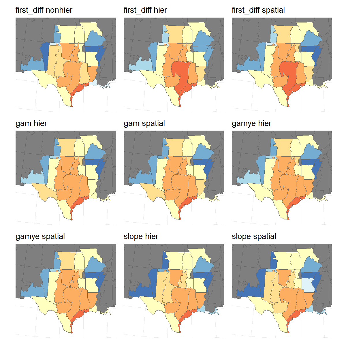

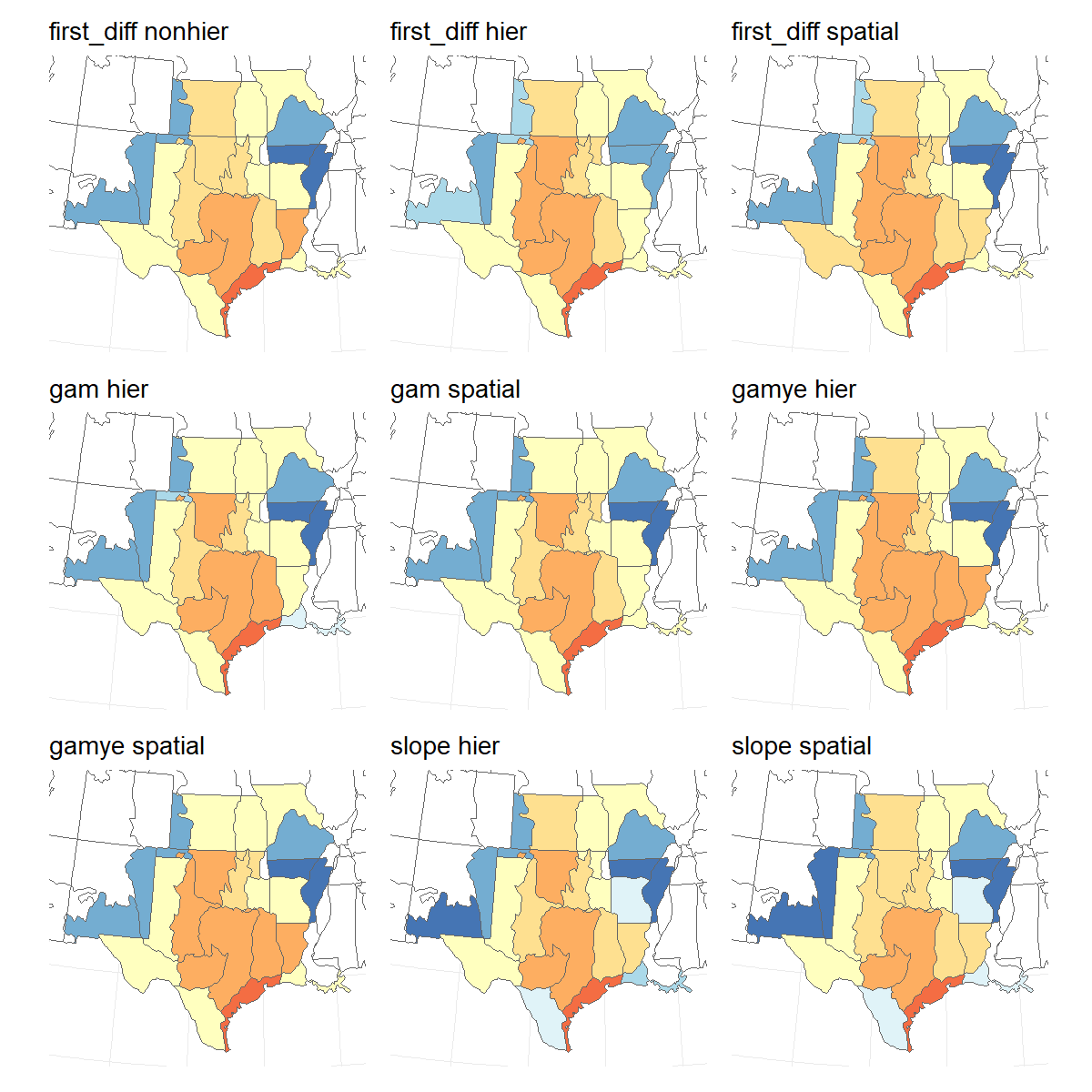
Similarly, the long-term trend maps are generally similar across the different models and variants.

map_panel <- patchwork::wrap_plots(saved_trend_maps,
                                    ncol = 3,
                                    guides = "collect")

print(map_panel)