library(bbsBayes2)
library(tidyverse)
#> Warning: package 'tidyverse' was built under R version 4.5.2
#> Warning: package 'ggplot2' was built under R version 4.5.2
Welcome!
bbsBayes2 is the successor to bbsBayes, with a major shift in functionality. The MCMC backend is now Stan instead of JAGS, the workflow has been streamlined, the syntax has changed, and there are new functions. This vignette should help you get started with the package, and there are three others that should help explain some of the new features, choices, and more advanced uses:
Stratification vignette The stratification vignette explains the built-in options for spatial stratifications as well as the workflow required to apply a custom stratification.
Models vignette The models vignette explains the four built-in models that differ in the way the temporal components are structured, and it also covers the built-in options for error distributions and the differences among the model variants (e.g.,
model_variant = "spatial").Advanced vignette The advanced vignette is helpful for users wanting to take the bbsBayes2 functionality further, including alternate calculations of population trend, customizing the Stan models, adding covariates, and even some experimental functions that allow for k-fold cross-validations and approximate leave-one-out calculations to compare fit and predictive accuracy among models.
First we’ll make sure we have the right software installed, we’ll fetch the BBS survey data, and then we’ll run through some example workflows.
Install bbsbayes2
If you haven’t already, install bbsBayes2 from the R-Universe.
install.packages("bbsBayes2", repos = c(bbsbayes = "https://bbsbayes.r-universe.dev",
                                        CRAN = getOption("repos")))
Note that due to non-CRAN dependencies, bbsBayes2 is not available on CRAN and must be installed from GitHub or the R-Universe.
Install cmdstanr
Because bbsBayes2 uses Stan to run the Bayesian models, we need to make sure we have cmdstanr and cmdstan both installed.
Run this in a fresh R session.
install.packages("cmdstanr", repos = c("https://mc-stan.org/r-packages/",
                                       getOption("repos")))
Now we should be able to use cmdstanr to install cmdstan
cmdstanr::install_cmdstan()Let’s check that everything went as planned, and tell cmdstanr to fix any issues.
cmdstanr::check_cmdstan_toolchain(fix = TRUE)
#> The C++ toolchain required for CmdStan is setup properly!
Problems? Check out cmdstanr’s vignette on Getting Started
Special note for Windows users
We strongly recommend that you install Linux on your Windows machine
and take advantage of cmdstanr functions that run
Stan models in Linux. This will likely cut the MCMC
run-times by 30-50% for the bbsBayes2 models. Installing Windows
Subsystem for Linux (WSL) is a small hassle, but only needs to be
done once. Follow the directions at the above link.
Once the WSL installation is complete, re-install
cmdstan using
cmdstanr::install_cmdstan(overwrite = TRUE, wsl = TRUE).
Now, everytime you run a model using cmdstan (and therefore
anytime you run a model using bbsBayes2), it will use the
Linux installation to run Stan. It’s seamless and you’ll be very
thankful you did it once it’s done.
Download BBS data
Now we’ll fetch the BBS data using the fetch_bbs_data()
function.
This will save the data to a package-specific directory on your
computer. You must agree to the terms and conditions of the data usage
before the download will run (type yes at the prompt). The
message also includes the key metadata for the dataset, including the
citation, acknowledgements, and the release-version (below). You only
need run this function once for each annual update of the BBS database
(these updates usually occur in the summer, approximately 1-year
following the data collection).
Note: Most bbsBayes2 functionality can be explored without downloading BBS data by using the included sample data. Specify
sample_data = TRUEin the firststratify()step (see the next section).
There are two types of BBS data that can be downloaded, and annual release-versions:
- Two levels
stateandstop(onlystateworks with bbsBayes2 models, thestopoption is provided to facilitate custom projects and models) - Annual releases
2020, and2022through2026more options will be added as annual releases occur).
The defaults (level state and the most recent release -
2026) is almost certainly what you are looking for, Unless
you have a specific reason to need a different version. The most recent
release will include all of the data included in earlier releases.
However you can download all releases and specify which one you wish to
use in the stratify() step.
A note about BBS release names:
The releases are named for the year in which the annual dataset was
released after going through QA-QC. So the 2022 release
contains all surveys conducted up to and including the 2021 field
season. There is no release = 2021, because the BBS was
cancelled during the COVID lockdowns of spring 2020 so no data were
collected and there was no updated data to release the following
year.
fetch_bbs_data()                  # Default - most recent release
fetch_bbs_data(release = "2020")  # Specify a different release
Workflow overview
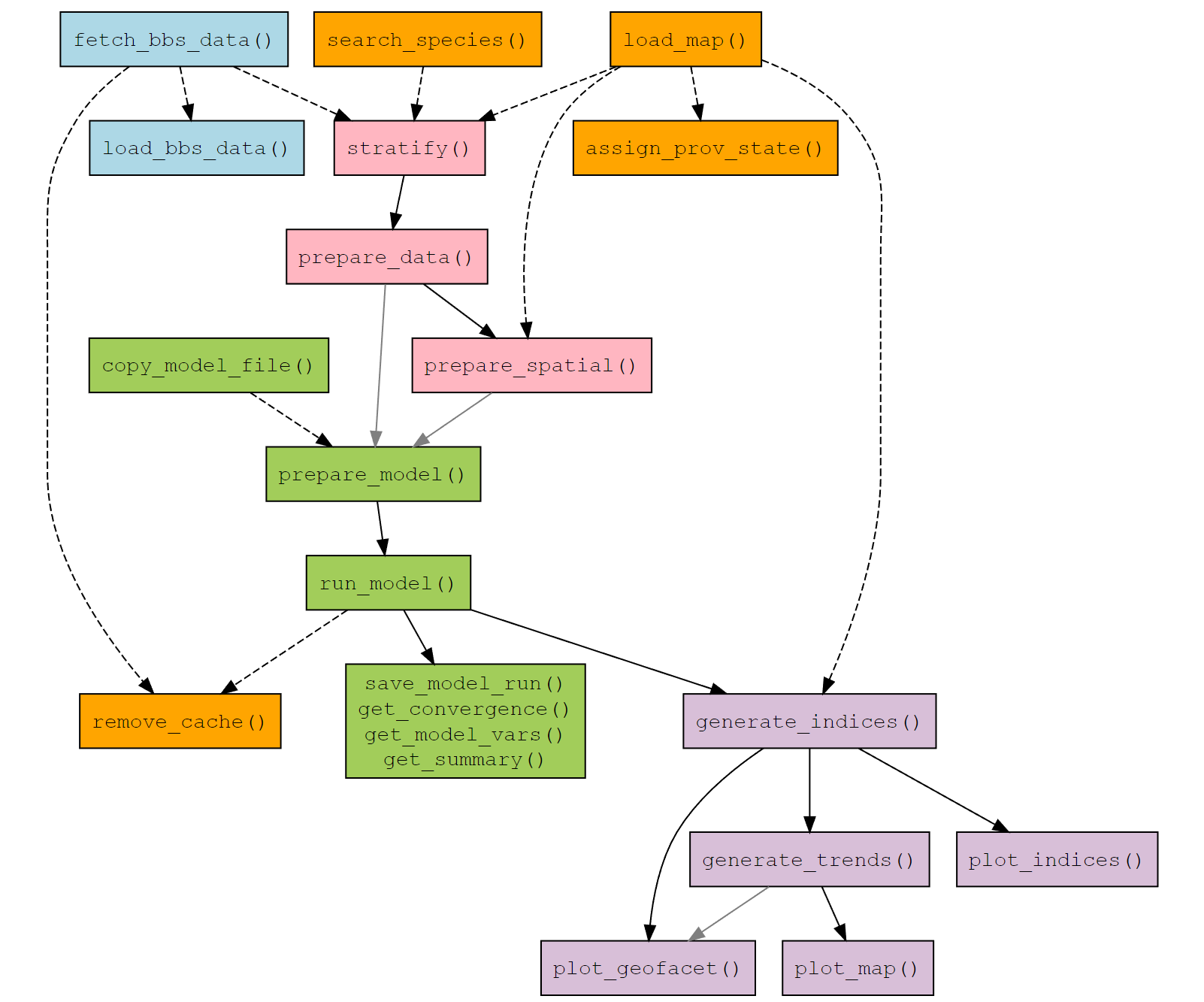
We can visualize the bbsBayes2 workflow with this flow chart of functions.
The functions are colour coded by category:
- BBS Data - Blue
- Data Prep - Pink
- Modelling - Green
- Exploring model trends and indices - Purple
- General helper functions - Orange
Functions which are connected by a solid, black
arrow, indicate that the output of the first function is required as
input to the second. For example, the output of stratify()
is required input for prepare_data().
Functions which are connected by a solid, grey
arrow, indicate that the output of the first function is
optional input to the second. For example, the output of
generate_trends() is an option input for
plot_geofacet().
Functions which are connected by a dotted arrow
indicate that the first function can be used to create input for the
second, but not necessarily directly. For example,
fetch_bbs_data() downloads BBS data which is used by
stratify(), but it isn’t an input. Alternatively,
load_map() can load a spatial data file for a specific
stratification which can be modified by the user and then used as input
to prepare_spatial() or
generate_indices().
See the Function Reference for more details on how to use a particular function.
Workflow to fit models
Note: If you would prefer to skip the model-fitting process for now, skip down to Workflow to explore the model outputs.
Now that you have cmdstanr installed and the BBS data downloaded, we’ll walk through a general workflow for modelling species trends with bbsBayes2.
Stratify the data
The first step in any bbsBayes2 analysis is to stratify the data. In this step we choose a stratification type as well as a species to explore.
s <- stratify(by = "bbs_usgs", species = "Scissor-tailed Flycatcher")
#> Using 'bbs_usgs' (standard) stratification
#> Loading BBS data...
#> Filtering to species Scissor-tailed Flycatcher (4430)
#> Stratifying data...
#> Preparing strata (ESRI:102008; North_America_Albers_Equal_Area_Conic)...
#>   Calculating area weights...
#>   Joining routes to spatial layer...
#>   Renaming routes...
#>   Omitting 2,489/130,138 surveys, on 111 unique routes that do not match a stratum.
#>     To see omitted routes use `return_omitted = TRUE` (see ?stratify)
We can also play around with the included sample data (Pacific Wrens)
s <- stratify(by = "bbs_cws", sample_data = TRUE) # Only Pacific Wren
#> Using 'bbs_cws' (standard) stratification
#> Using sample BBS data...
#> Using species Pacific Wren (sample data)
#> Filtering to species Pacific Wren (7221)
#> Stratifying data...
#> Preparing strata (ESRI:102008; North_America_Albers_Equal_Area_Conic)...
#>   Calculating area weights...
#>   Joining routes to spatial layer...
#>   Renaming routes...
#>   Omitting 503/5,480 surveys, on 25 unique routes that do not match a stratum.
#>     To see omitted routes use `return_omitted = TRUE` (see ?stratify)
Stratifications included in bbsBayes2 are bbs, bbs_usgs, bbs_cws, bcr, bcr_old, latlong, prov_state. See the article on stratifications for more details and examples.
Species names in bbsBayes2
Let’s first take a brief step out of the workflow to explain important information about species names in bbsBayes2.
All of the models in the package are species-specific. So the species
is a fundamental aspect of any analysis. The
search_species() function allows the user to search up the
species names in the BBS database, using text from the English, Spanish,
French, or Latin names. The English names for each species will be
retained in the metadata at every step of the workflow.
search_species("Geai bleu")
#> # A tibble: 1 × 8
#>     aou english  french    order         family   genus      species  unid_combined
#>   <dbl> <chr>    <chr>     <chr>         <chr>    <chr>      <chr>    <lgl>
#> 1  4770 Blue Jay Geai bleu Passeriformes Corvidae Cyanocitta cristata TRUE
search_species("Cyanocitta")
#> # A tibble: 2 × 8
#>     aou english       french          order         family   genus      species  unid_combined
#>   <dbl> <chr>         <chr>           <chr>         <chr>    <chr>      <chr>    <lgl>
#> 1  4780 Steller's Jay Geai de Steller Passeriformes Corvidae Cyanocitta stelleri TRUE
#> 2  4770 Blue Jay      Geai bleu       Passeriformes Corvidae Cyanocitta cristata TRUE
search_species("Corvidae")
#> # A tibble: 20 × 8
#>      aou english                                            french                    order family genus species unid_combined
#>    <dbl> <chr>                                              <chr>                     <chr> <chr>  <chr> <chr>   <lgl>
#>  1  4840 Canada Jay                                         Mésangeai du Canada       Pass… Corvi… Peri… canade… TRUE
#>  2  4830 Green Jay                                          Geai vert                 Pass… Corvi… Cyan… yncas   TRUE
#>  3  4920 Pinyon Jay                                         Geai des pinèdes          Pass… Corvi… Gymn… cyanoc… TRUE
#>  4  4780 Steller's Jay                                      Geai de Steller           Pass… Corvi… Cyan… stelle… TRUE
#>  5  4770 Blue Jay                                           Geai bleu                 Pass… Corvi… Cyan… crista… TRUE
#>  6  4790 Florida Scrub-Jay                                  Geai à gorge blanche      Pass… Corvi… Aphe… coerul… TRUE
#>  7  4811 Island Scrub-Jay                                   Geai de Santa Cruz        Pass… Corvi… Aphe… insula… TRUE
#>  8  4812 California Scrub-Jay                               Geai buissonnier          Pass… Corvi… Aphe… califo… TRUE
#>  9  4813 Woodhouse's Scrub-Jay                              Geai de Woodhouse         Pass… Corvi… Aphe… woodho… TRUE
#> 10  4810 unid. California Scrub-Jay / Woodhouse's Scrub-Jay unid Geai buissonnier / … Pass… Corvi… Aphe… califo… TRUE
#> 11  4820 Mexican Jay                                        Geai du Mexique           Pass… Corvi… Aphe… wollwe… TRUE
#> 12  4910 Clark's Nutcracker                                 Cassenoix d'Amérique      Pass… Corvi… Nuci… columb… TRUE
#> 13  4750 Black-billed Magpie                                Pie d'Amérique            Pass… Corvi… Pica  hudson… TRUE
#> 14  4760 Yellow-billed Magpie                               Pie à bec jaune           Pass… Corvi… Pica  nuttal… TRUE
#> 15  4880 American Crow                                      Corneille d'Amérique      Pass… Corvi… Corv… brachy… TRUE
#> 16  4900 Fish Crow                                          Corneille de rivage       Pass… Corvi… Corv… ossifr… TRUE
#> 17  4881 unid. American Crow / Fish Crow                    unid Corneille d'Amériqu… Pass… Corvi… Corv… brachy… TRUE
#> 18  4870 Chihuahuan Raven                                   Corbeau à cou blanc       Pass… Corvi… Corv… crypto… TRUE
#> 19  4860 Common Raven                                       Grand Corbeau             Pass… Corvi… Corv… corax   TRUE
#> 20  4865 unid. Chihuahuan Raven / Common Raven              unid Grand Corbeau / Cor… Pass… Corvi… Corv… crypto… TRUE
Species groupings
There are some taxonomic groupings of species-units in the BBS database that bbsBayes2 by default also groups into combined species forms. These represent groupings that make sense based on changes in taxonomy or potentially inconsistent distinctions among observers, routes, regions, or time.
- There are groupings that represent species considered distinct in the early portion of the BBS history that have been lumped into a single species at some point since then. For example, the Northern Flicker observations exist in the BBS database separately as Red-shafted Flicker (4130), Yellow-shafted Flicker (4120), unidentified Red/Yellow-shafted Flicker (4123) or hybrid Red x Yellow-shafted Flicker (4125). To provide an appropriate dataset to represent population trends of Northern Flicker, bbsBayes2 by default sums all of these observations into a new species called Northern Flicker (all forms), which replaces the (4123) unidentified category in the species database. The remaining original separate forms (Red, Yellow, and hybrid) are retained.
- Similar combined species are created for taxonomic splits that have occurred since the start of the BBS, such as Clark’s and Western Grebe, which are retained as their own separate species, but are also combined into Western Grebe (Clark’s/Western) (12). You can access a complete list of these combined species groups and the sub groups that make them up.
bbsBayes2::species_forms
#>    aou_unid                               english_original                                   english_combined
#> 1      2973              unid. Dusky Grouse / Sooty Grouse                          Blue Grouse (Dusky/Sooty)
#> 2      5677                   (unid. race) Dark-eyed Junco                        Dark-eyed Junco (all forms)
#> 3      4123    (unid. Red/Yellow Shafted) Northern Flicker                       Northern Flicker (all forms)
#> 4      5077      unid. Bullock's Oriole / Baltimore Oriole              Northern Oriole (Bullock's/Baltimore)
#> 5      3370                                Red-tailed Hawk                        Red-tailed Hawk (all forms)
#> 6      4022                                unid. sapsucker Sapsuckers (Yellow-bellied/Red-naped/Red-breasted)
#> 7      1690                                     Snow Goose                             Snow Goose (all forms)
#> 8      6295       unid. Cassin's Vireo / Blue-headed Vireo              Solitary Vireo (Blue-headed/Cassin's)
#> 9      4665     unid. Alder Flycatcher / Willow Flycatcher                 Traill's Flycatcher (Alder/Willow)
#> 10     4642   unid. Cordilleran / Pacific-slope Flycatcher     Western Flycatcher (Cordilleran/Pacific-slope)
#> 11       12            unid. Western Grebe / Clark's Grebe                    Western Grebe (Clark's/Western)
#> 12     6556 (unid. Myrtle/Audubon's) Yellow-rumped Warbler                  Yellow-rumped Warbler (all forms)
#> 13     5275           unid. Common Redpoll / Hoary Redpoll                             Redpoll (Common/Hoary)
#> 14     5012                               unid. Meadowlark            Meadowlark (Eastern/Western/Chihuahuan)
#>                                                french_combined                       aou_id
#> 1                            Tétras sombre (sombre/fuligineux)                   2970, 2971
#> 2                            Junco ardoisé (toutes les formes) 5671, 5670, 5680, 5660, 5690
#> 3                           Pic flamboyant (toutes les formes)             4125, 4120, 4130
#> 4                     Oriole du Nord (de Bullock/de Baltimore)             5080, 5070, 5078
#> 5                      Buse à queue rousse (toutes les formes)                         3380
#> 6  Pics buveur de sève (maculé/à nuque rouge/à poitrine rouge)       4020, 4021, 4031, 4032
#> 7                           Oie des neiges (toutes les formes)                         1691
#> 8                  Viréo à tête bleue (à tête bleue/de Cassin)             6292, 6291, 6290
#> 9               Moucherolle de Traill (des aulnes/ des saules)                   4661, 4660
#> 10                     Moucherolle côtier (des ravins/ côtier)                   4641, 4640
#> 11                      Grèbe élégant (à face blanche/élégant)                       10, 11
#> 12               Paruline à croupion jaune (toutes les formes)                   6550, 6560
#> 13                                 Sizerin (flammé/blanchâtre)                   5270, 5280
#> 14 Sturnelle (prés/Ouest/Lilian) 5009, 5010, 5011- These splits that have occurred since the start of the BBS require
some extra care when considering what years to include in any model fit.
For example, if fitting a trend model to the data for Clark’s Grebe, it
would not make sense to include all years back to 1966. Prior to 1985,
Clark’s Grebe was not a distinct species and so observers would not have
recorded observations for this species in the same was as they
would have after 1985. The
prepare_data()function will generate warnings if the user selects a species and time-period where these species identification-issues may be important. Related concerns with time-span may apply to species that have expanded their range into the surveyed area of the BBS since the beginning of surveys. A list of the species where these time-span concerns may be most relevant can be found by calling the built-in data table.
bbsBayes2::species_notes
#>                  english                  french   aou minimum_year
#> 1       Alder Flycatcher  Moucherolle des aulnes  4661         1978
#> 2      Willow Flycatcher  Moucherolle des saules  4660         1978
#> 3          Clark's Grebe    Grèbe à face blanche    11         1990
#> 4          Western Grebe           Grèbe élégant    10         1990
#> 5 Eurasian Collared-Dove      Tourterelle turque 22860         1990
#> 6           Cave Swallow Hirondelle à front brun  6121         1985
#>                                                                                                                                                                                     warning
#> 1 Alder and Willow Flycatcher were considered a single species until 1973. It is likely that they are not accurately separated by BBS observers until at least some years after that split.
#> 2 Alder and Willow Flycatcher were considered a single species until 1973. It is likely that they are not accurately separated by BBS observers until at least some years after that split.
#> 3   Clark's and Western Grebe were considered a single species until 1985. It is likely that they are not accurately separated by BBS observers until at least some years after that split.
#> 4   Clark's and Western Grebe were considered a single species until 1985. It is likely that they are not accurately separated by BBS observers until at least some years after that split.
#> 5                                     Eurasian Collared Dove was introduced into North America in the 1980s. 1990 is the first year that the species was observed on at least 3 BBS routes.
#> 6                                                      Cave Swallows were relatively rare in the areas surveyed by BBS before 1980. There are only two observations during BBS before 1980.
If you’re looking for a complete list of all species in the BBS database.
all_species_bbs_database <- load_bbs_data()$speciesNote: Because models can take hours to days to run, if you’re exploring the package functionality, we recommend using species with relatively small ranges (i.e., relatively few data) such as the Hepatic Tanager, Pacific Wren, or Scissor-tailed Flycatcher.
Prepare the data
Once we have stratified the data, we can now prepare it for use in a
model. In this step data will be filtered to omit routes with too few
samples, etc. See prepare_data() for more details on how
you can customize this step.
p <- prepare_data(s)Prepare the model
Next we will prepare the model parameters and initialization values.
See prepare_model() for more details on how you can
customize this step.
md <- prepare_model(p, model = "first_diff")Run model
Now we can run the model.
The default iter_sampling and iter_warmup
are 1000 and the default chains is 4. In the interest of
speed for this example, we are using much lower values, but note that
this almost certainly will result in problems with our model.
m <- run_model(md, iter_sampling = 100, iter_warmup = 500, chains = 2)Additional steps for spatial models
For spatial models there are two additional steps. You stratify and prepare the data as in the previous example, but you also prepare the map and the spatial data. An example is below.
s <- stratify(by = "bbs_usgs", species="Scissor-tailed Flycatcher")
#> Using 'bbs_usgs' (standard) stratification
#> Loading BBS data...
#> Filtering to species Scissor-tailed Flycatcher (4430)
#> Stratifying data...
#> Preparing strata (ESRI:102008; North_America_Albers_Equal_Area_Conic)...
#>   Calculating area weights...
#>   Joining routes to spatial layer...
#>   Renaming routes...
#>   Omitting 2,489/130,138 surveys, on 111 unique routes that do not match a stratum.
#>     To see omitted routes use `return_omitted = TRUE` (see ?stratify)
p <- prepare_data(s)
And now the additional steps…
# Load a map
map <- load_map(stratify_by = "bbs_usgs")
# Prepare the spatial data
sp <- prepare_spatial(p, map)
#> Preparing spatial data...
#> Identifying neighbours (non-Voronoi method)...
#> Formating neighbourhood matrices...
#> Plotting neighbourhood matrices...
Then the remaining steps are the same but we use
model_variant = "spatial" in
prepare_model().
# Then prepare the model with the spatial output
mod <- prepare_model(sp, model = "gamye", model_variant = "spatial")

# Then run the model as before
m <- run_model(mod)

# Optionally, save the model output as an .rds file
saveRDS(m, "output/4430_gamye_spatial.rds")
The spatial aspects of the spatial model variants use an intrinsic Conditional Autoregressive structure (iCAR) to share information among neighbouring strata on the population abundance and trend parameter (Besag et al. 1991, ver Hoef et al. 2018, Morris et al. 2019). For more information about the bbsBayes2 models and the spatial models see the models vignette and Smith et al., 2024.
The prepared spatial data object includes a map of the spatial neighbourhood relationships for a given species and stratification.
print(sp$spatial_data$map)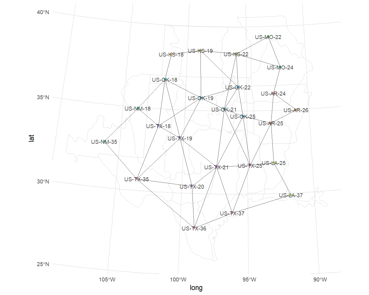
Workflow to explore the model outputs
If you would prefer to skip the model fitting steps for now, you can download a fitted model object (the output of the code below) and test out the remaining package features.
library(bbsBayes2)
library(tidyverse)

species <- "Scissor-tailed Flycatcher"

# extract the unique numerical identifier for this species in the BBS database
species_number <- search_species(species) %>%
  select(aou) %>%
  unlist()

mod <- "gamye"
var <- "spatial"

out_name <- paste0("output/",
                      species_number,
                      "_",
                      mod,
                      "_",
                      var)

d <- stratify("bbs_usgs",
              species = species) %>%
  prepare_data() %>%
  prepare_spatial(s, strata_map = load_map("bbs_usgs")) %>%
  prepare_model(model = mod, model_variant = var)

m <- run_model(d,
    output_basename = out_name,
    output_dir = getwd()) # by default saves the model output using output_basename
The outputs of the collection of functions required to fit a model
are cumulative: each one retains the metadata from the previous step. As
a result, the saved object from the run_model() function is
a large list that includes the cmdstanr posterior samples
object from the model fitting process, as well as all of the data and
metadata necessary to understand and replicate the choices made to fit
the model.
m <- readRDS("output/4430_gamye_spatial.rds")
names(m)
#> [1] "model_fit"   "model_data"  "meta_data"   "meta_strata" "raw_data"
Convergence and parameter summaries
First, we will investigate the model convergence and the parameter
estimates of the model. There are two key helper functions in
bbsBayes2 that provide information on model convergence:
get_convergence() calculates convergence diagnostics and
get_summary() calculates the convergence diagnostics as
well as summary statistics (mean, median, credible intervals) for all
parameters in a fitted model.
# Convergence diagnostics for all parameters
converge <- get_convergence(m)
# Convergence diagnostics for all smoothed annual indices
converge_n_smooth <- get_convergence(m, variables = "n_smooth") %>%
  arrange(-rhat)
converge_n_smooth
#> # A tibble: 1,508 × 5
#>    variable_type variable         rhat ess_bulk ess_tail
#>    <chr>         <chr>           <dbl>    <dbl>    <dbl>
#>  1 n_smooth      n_smooth[22,33]  1.00    5336.    3849.
#>  2 n_smooth      n_smooth[20,47]  1.00    5026.    4011.
#>  3 n_smooth      n_smooth[15,35]  1.00    5596.    3152.
#>  4 n_smooth      n_smooth[15,33]  1.00    5680.    3508.
#>  5 n_smooth      n_smooth[8,1]    1.00    4823.    3289.
#>  6 n_smooth      n_smooth[22,32]  1.00    5323.    3855.
#>  7 n_smooth      n_smooth[14,13]  1.00    5787.    3749.
#>  8 n_smooth      n_smooth[15,34]  1.00    5641.    3408.
#>  9 n_smooth      n_smooth[20,46]  1.00    5222.    4099.
#> 10 n_smooth      n_smooth[7,20]   1.00    5197.    3682.
#> # ℹ 1,498 more rows
Here we’ve sorted the convergence diagnostics by rhat values (highest
values at the top to highlight any problems). Cut-offs for rhat
statistics are somewhat arbitrary and recommendations vary in the
literature, but values of rhat > 1.1 indicate a very serious
problem with the convergence of some of the parameters in the model
(i.e., there is more variation among the independent chains than within
them) and values of ess_bulk < ~400 suggest an imprecise estimate of
the parameter. In some cases, refitting the model with more iterations
(both warmup and sampling) may improve convergence. More advice on
exploring Bayesian model convergence can be found in Gabry et al., 2019.
bbsBayes2 relies on functions in the packages cmdstanr and
posterior to calculate rhat values following Vehtari et al. 2021.
m <- run_model(mod,
               iter_warmup = 2000,
               iter_sampling = 2000)
It is possible to thin the MCMC chains by passing arguments from
cmdstanr::sample() into the run_model()
function. The call below would result in the same number of posterior
samples as run_model() defaults, but may improve the
efficiency of the sampling (and of course would also increase the time
required to fit the model by a factor of approximately 4).
m <- run_model(mod,
               iter_warmup = 4000,
               iter_sampling = 4000,
               thin = 4)
If you want summary statistics of the parameters, as well as
convergence diagnostics, the function get_summary() may be
more useful.
# Summary statistics and convergence diagnostics for all parameters
summary_stats <- get_summary(m)
# Summary statistics and convergence diagnostics for all smoothed annual indices
summary_stats_n_smooth <- get_summary(m, variables = "n_smooth") %>%
  arrange(-rhat)
summary_stats_n_smooth
#> # A tibble: 1,508 × 11
#>    variable_type variable          mean median    sd   mad     q5    q95  rhat ess_bulk ess_tail
#>    <chr>         <chr>            <dbl>  <dbl> <dbl> <dbl>  <dbl>  <dbl> <dbl>    <dbl>    <dbl>
#>  1 n_smooth      n_smooth[22,33] 28.4   28.4   1.01  0.987 26.8   30.1    1.00    5336.    3849.
#>  2 n_smooth      n_smooth[20,47] 28.5   28.5   1.65  1.64  25.9   31.3    1.00    5026.    4011.
#>  3 n_smooth      n_smooth[15,35] 19.5   19.5   1.24  1.23  17.6   21.6    1.00    5596.    3152.
#>  4 n_smooth      n_smooth[15,33] 17.7   17.6   1.12  1.10  15.9   19.6    1.00    5680.    3508.
#>  5 n_smooth      n_smooth[8,1]    0.294  0.271 0.120 0.103  0.144  0.517  1.00    4823.    3289.
#>  6 n_smooth      n_smooth[22,32] 28.4   28.4   1.00  0.967 26.8   30.0    1.00    5323.    3855.
#>  7 n_smooth      n_smooth[14,13] 18.6   18.6   1.09  1.08  16.9   20.5    1.00    5787.    3749.
#>  8 n_smooth      n_smooth[15,34] 18.6   18.5   1.18  1.17  16.7   20.5    1.00    5641.    3408.
#>  9 n_smooth      n_smooth[20,46] 28.1   28.0   1.62  1.62  25.5   30.8    1.00    5222.    4099.
#> 10 n_smooth      n_smooth[7,20]   0.729  0.718 0.122 0.120  0.549  0.942  1.00    5197.    3682.
#> # ℹ 1,498 more rows
Indices - predictions of annual relative abundance
Indices (annual indices of relative abundance) represent mean
predicted annual counts of the species in a given region, on an average
route, by an average observer. The pattern in the time-series of these
annual indices for a given region represent the estimated population
trajectory. We generate indices according to different categories of
regional summaries. All of the bbsBayes2 models are stratified based on
geographic spatial units, and these categories of regions are either
these strata (generate_indices(region = "stratum")), or
some combination of strata. By default the selected regions for most
model summaries are continent and stratum. The
continent estimates represent the area- and
abundance-weighted means across all strata, other regional summaries are
built in for some stratifications that allow it (e.g.,
region = "country" for the stratifications
bbs_usgs, bbs_cws, or
prov_state).
i <- generate_indices(model_output = m)
#> Processing region continent
#> Processing region stratum
We can explore or extract these indices for saving as an external
file (e.g., export to .csv), by accessing the indices item
in the list.
i[["indices"]]
#> # A tibble: 1,566 × 17
#>     year region    region_type strata_included      strata_excluded index index_q_0.025 index_q_0.05 index_q_0.25 index_q_0.75
#>    <dbl> <chr>     <chr>       <chr>                <chr>           <dbl>         <dbl>        <dbl>        <dbl>        <dbl>
#>  1  1967 continent continent   US-AR-24 ; US-AR-25… ""              13.5          12.1         12.3         13.0          14.0
#>  2  1968 continent continent   US-AR-24 ; US-AR-25… ""              13.5          12.2         12.4         13.0          13.9
#>  3  1969 continent continent   US-AR-24 ; US-AR-25… ""              13.4          12.3         12.5         13.0          13.8
#>  4  1970 continent continent   US-AR-24 ; US-AR-25… ""              13.5          12.5         12.6         13.2          13.9
#>  5  1971 continent continent   US-AR-24 ; US-AR-25… ""              13.4          12.5         12.6         13.0          13.7
#>  6  1972 continent continent   US-AR-24 ; US-AR-25… ""              13.2          12.4         12.5         12.9          13.6
#>  7  1973 continent continent   US-AR-24 ; US-AR-25… ""              12.1          11.3         11.4         11.8          12.4
#>  8  1974 continent continent   US-AR-24 ; US-AR-25… ""              11.4          10.7         10.8         11.2          11.7
#>  9  1975 continent continent   US-AR-24 ; US-AR-25… ""              10.7          10.0         10.1         10.5          11.0
#> 10  1976 continent continent   US-AR-24 ; US-AR-25… ""               9.84          9.19         9.29         9.60         10.1
#> # ℹ 1,556 more rows
#> # ℹ 7 more variables: index_q_0.95 <dbl>, index_q_0.975 <dbl>, obs_mean <dbl>, n_routes <int>, n_routes_total <int>,
#> #   n_non_zero <int>, backcast_flag <dbl>
Trajectory plots
We can also generate time-series plots of these indices to visualize population trajectories.
# generates a list of ggplot graphs, one for each region
p <- plot_indices(indices = i,
                  add_observed_means = TRUE) # optional argument to show raw observed mean counts
Note that we get one plot for each region and regional category, in this case that means one plot for the continent, and one for each stratum.
names(p)
#>  [1] "continent" "US_AR_24"  "US_AR_25"  "US_AR_26"  "US_KS_18"  "US_KS_19"  "US_KS_22"  "US_LA_25"  "US_LA_37"  "US_MO_22"
#> [11] "US_MO_24"  "US_NM_18"  "US_NM_35"  "US_OK_18"  "US_OK_19"  "US_OK_21"  "US_OK_22"  "US_OK_24"  "US_OK_25"  "US_TX_18"
#> [21] "US_TX_19"  "US_TX_20"  "US_TX_21"  "US_TX_25"  "US_TX_35"  "US_TX_36"  "US_TX_37"
We can plot them individually by pulling a plot out of the list
print(p[["continent"]])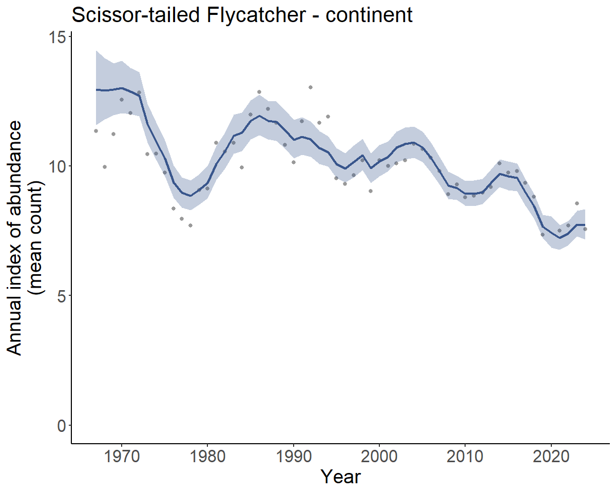
Each of these plots is a ggplot2 object that can be modified like any other. For example, you can modify titles or axes.
library(ggplot2)

p1_mod <- p[["continent"]]+
  coord_cartesian(xlim = c(2000,NA))+ #subset of years
  labs(title = "") # remove the title
print(p1_mod)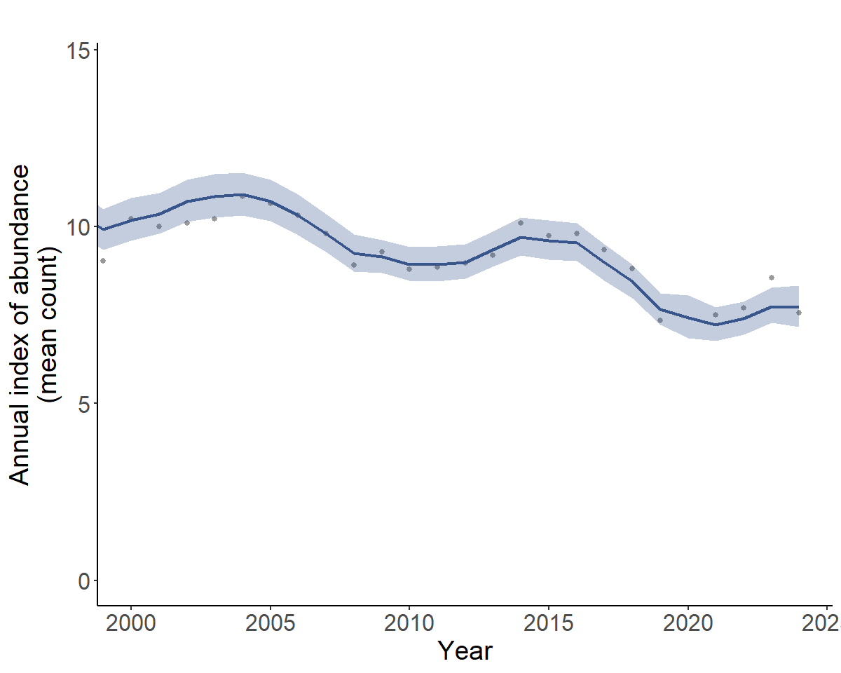
Spaghetti plots to show uncertainty in population trajectories
The most common inference to draw from one of these BBS models
relates to the estimates of the population trajectory. One particularly
useful way to visualise the uncertainty of those population trajectories
is to plot many posterior draws of the full trajectory. The default
population trajectories plots plot_indices() show a line
representing the path of the annual posterior medians of the annual
indices and an uncertainty band spanning the outer limits of a credible
interval on the annual indices. These are reasonable summaries of the
uncertainty in the collection of annual indices. However, the
uncertainty of each annual index of abundance includes information about
the uncertainty in the estimate of the change in abundance through time
(e.g., trend) and uncertainty in the estimate of the mean abundance
(e.g., the mean count in any given route or observer). Those two sources
of uncertainty can be correlated in the posterior distribution, so that
the uncertainty of the annual indices may over-estimate the uncertainty
in the trend. To plot a sample of estimated trajectories, set the
spaghetti = TRUE argument in the
plot_indices() function.
# generates a list of ggplot graphs, one for each region
p <- plot_indices(indices = i,
add_observed_means = TRUE,
spaghetti = TRUE)
print(p[["continent"]])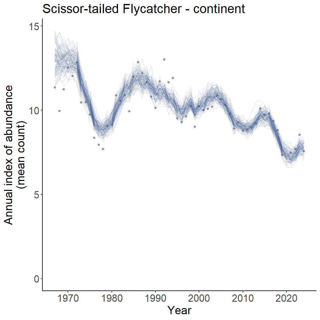 There are arguments that also allow the user to control the transparency
of each plotted line, as well as the number of lines to plot (the
default is to draw 100 random samples).
There are arguments that also allow the user to control the transparency
of each plotted line, as well as the number of lines to plot (the
default is to draw 100 random samples).
Trends - predictions of mean rates of change over time
Next we can calculate the long-term trends based on these indices. Note all trends from bbsBayes2 models are derived from summaries of indices through time or between two points in time.
t <- generate_trends(i)We can explore or extract these trends for saving as an external file
(e.g., export to .csv), by accessing the trends item in the
list.
t[["trends"]]
#> # A tibble: 27 × 27
#>    start_year end_year region    region_type strata_included   strata_excluded   trend trend_q_0.025 trend_q_0.05 trend_q_0.25
#>         <dbl>    <dbl> <chr>     <chr>       <chr>             <chr>             <dbl>         <dbl>        <dbl>        <dbl>
#>  1       1967     2024 continent continent   US-AR-24 ; US-AR… ""              -0.965         -1.22        -1.18       -1.05
#>  2       1967     2024 US-AR-24  stratum     US-AR-24          ""               4.81           3.75         3.91        4.43
#>  3       1967     2024 US-AR-25  stratum     US-AR-25          ""              -0.304         -1.10        -0.946      -0.554
#>  4       1967     2024 US-AR-26  stratum     US-AR-26          ""               3.40           1.15         1.54        2.63
#>  5       1967     2024 US-KS-18  stratum     US-KS-18          ""               2.75          -1.33        -0.650       1.29
#>  6       1967     2024 US-KS-19  stratum     US-KS-19          ""              -0.458         -1.23        -1.11       -0.723
#>  7       1967     2024 US-KS-22  stratum     US-KS-22          ""              -0.0114        -0.691       -0.587      -0.249
#>  8       1967     2024 US-LA-25  stratum     US-LA-25          ""              -1.21          -2.79        -2.55       -1.73
#>  9       1967     2024 US-LA-37  stratum     US-LA-37          ""               0.301         -1.81        -1.47       -0.385
#> 10       1967     2024 US-MO-22  stratum     US-MO-22          ""               0.655         -0.979       -0.707       0.0825
#> # ℹ 17 more rows
#> # ℹ 17 more variables: trend_q_0.75 <dbl>, trend_q_0.95 <dbl>, trend_q_0.975 <dbl>, percent_change <dbl>,
#> #   percent_change_q_0.025 <dbl>, percent_change_q_0.05 <dbl>, percent_change_q_0.25 <dbl>, percent_change_q_0.75 <dbl>,
#> #   percent_change_q_0.95 <dbl>, percent_change_q_0.975 <dbl>, width_of_95_percent_credible_interval <dbl>,
#> #   rel_abundance <dbl>, obs_rel_abundance <dbl>, n_routes <dbl>, mean_n_routes <dbl>, n_strata_included <dbl>,
#> #   backcast_flag <dbl>
We can generate trends for different periods of time, using any
combination of a starting year min_year and ending year
max_year.
t_10 <- generate_trends(i,
min_year = 2011,
max_year = 2021)
t_10
#> $trends
#> # A tibble: 27 × 27
#> start_year end_year region region_type strata_included strata_excluded trend trend_q_0.025 trend_q_0.05 trend_q_0.25
#> <dbl> <dbl> <chr> <chr> <chr> <chr> <dbl> <dbl> <dbl> <dbl>
#> 1 2011 2021 continent continent US-AR-24 ; US-AR-… "" -2.15 -2.90 -2.77 -2.40
#> 2 2011 2021 US-AR-24 stratum US-AR-24 "" 1.78 -0.972 -0.528 0.831
#> 3 2011 2021 US-AR-25 stratum US-AR-25 "" -0.634 -3.17 -2.67 -1.44
#> 4 2011 2021 US-AR-26 stratum US-AR-26 "" 4.23 -1.20 -0.360 2.39
#> 5 2011 2021 US-KS-18 stratum US-KS-18 "" 3.06 -3.01 -2.05 1.02
#> 6 2011 2021 US-KS-19 stratum US-KS-19 "" 0.602 -2.23 -1.76 -0.395
#> 7 2011 2021 US-KS-22 stratum US-KS-22 "" -3.80 -6.11 -5.67 -4.57
#> 8 2011 2021 US-LA-25 stratum US-LA-25 "" -1.94 -8.71 -7.74 -4.23
#> 9 2011 2021 US-LA-37 stratum US-LA-37 "" 1.81 -4.87 -3.96 -0.768
#> 10 2011 2021 US-MO-22 stratum US-MO-22 "" -2.19 -6.90 -6.02 -3.81
#> # ℹ 17 more rows
#> # ℹ 17 more variables: trend_q_0.75 <dbl>, trend_q_0.95 <dbl>, trend_q_0.975 <dbl>, percent_change <dbl>,
#> # percent_change_q_0.025 <dbl>, percent_change_q_0.05 <dbl>, percent_change_q_0.25 <dbl>, percent_change_q_0.75 <dbl>,
#> # percent_change_q_0.95 <dbl>, percent_change_q_0.975 <dbl>, width_of_95_percent_credible_interval <dbl>,
#> # rel_abundance <dbl>, obs_rel_abundance <dbl>, n_routes <dbl>, mean_n_routes <dbl>, n_strata_included <dbl>,
#> # backcast_flag <dbl>
#>
#> $meta_data
#> $meta_data$stratify_by
#> [1] "bbs"
#>
#> $meta_data$stratify_type
#> [1] "standard"
#>
#> $meta_data$species
#> [1] "Scissor-tailed Flycatcher"
#>
#> $meta_data$sp_aou
#> [1] 4430
#>
#> $meta_data$model
#> [1] "gamye"
#>
#> $meta_data$model_variant
#> [1] "spatial"
#>
#> $meta_data$model_file
#> [1] "C:/Users/SmithAC/AppData/Local/R/win-library/4.5/bbsBayes2/models/gamye_spatial_bbs_CV.stan"
#>
#> $meta_data$run_date
#> [1] "2026-01-28 00:14:49 EST"
#>
#> $meta_data$bbsBayes2_version
#> [1] "1.1.3.2"
#>
#> $meta_data$cmdstan_path
#> [1] "//wsl$/ECCC-WSL-UBUNTU-24/home/acsmith/.cmdstan/cmdstan-2.37.0"
#>
#> $meta_data$cmdstan_version
#> [1] "2.37.0"
#>
#> $meta_data$regions
#> [1] "continent" "stratum"
#>
#> $meta_data$start_year
#> [1] 1967
#>
#> $meta_data$n_years
#> [1] 58
#>
#> $meta_data$hpdi_indices
#> [1] FALSE
#>
#> $meta_data$hpdi_trends
#> [1] FALSE
#>
#> $meta_data$gam_smooth_trends
#> [1] FALSE
#>
#>
#> $meta_strata
#> # A tibble: 26 × 5
#> strata_name strata area_sq_km continent stratum
#> <chr> <dbl> <dbl> <chr> <chr>
#> 1 US-AR-24 1 33282. continent US-AR-24
#> 2 US-AR-25 2 65413. continent US-AR-25
#> 3 US-AR-26 3 38825. continent US-AR-26
#> 4 US-KS-18 4 36499. continent US-KS-18
#> 5 US-KS-19 5 109257. continent US-KS-19
#> 6 US-KS-22 6 65859. continent US-KS-22
#> 7 US-LA-25 7 47058. continent US-LA-25
#> 8 US-LA-37 8 27890. continent US-LA-37
#> 9 US-MO-22 9 83314. continent US-MO-22
#> 10 US-MO-24 10 86717. continent US-MO-24
#> # ℹ 16 more rows
#>
#> $raw_data
#> # A tibble: 13,485 × 27
#> country_num state_num state rpid bcr year strata_name route obs_n latitude longitude route_data_id run_type count
#> <dbl> <dbl> <chr> <dbl> <dbl> <dbl> <chr> <chr> <dbl> <dbl> <dbl> <dbl> <dbl> <dbl>
#> 1 840 7 ARKANSAS 101 26 1969 US-AR-24 7-19 1070050 35.9 -91.3 6167138 1 0
#> 2 840 7 ARKANSAS 101 26 1971 US-AR-24 7-19 1070050 35.9 -91.3 6168780 1 0
#> 3 840 7 ARKANSAS 101 26 1972 US-AR-24 7-19 1070050 35.9 -91.3 6174037 1 0
#> 4 840 7 ARKANSAS 101 26 1973 US-AR-24 7-19 1070050 35.9 -91.3 6174466 1 0
#> 5 840 7 ARKANSAS 101 26 1975 US-AR-24 7-19 1070050 35.9 -91.3 6179441 1 0
#> 6 840 7 ARKANSAS 101 26 1977 US-AR-24 7-19 1080130 35.9 -91.3 6183099 1 0
#> 7 840 7 ARKANSAS 101 26 1978 US-AR-24 7-19 1080130 35.9 -91.3 6187774 1 0
#> 8 840 7 ARKANSAS 101 26 1979 US-AR-24 7-19 1040020 35.9 -91.3 6185565 1 0
#> 9 840 7 ARKANSAS 101 26 1980 US-AR-24 7-19 1040020 35.9 -91.3 6186949 1 0
#> 10 840 7 ARKANSAS 101 26 1981 US-AR-24 7-19 1040020 35.9 -91.3 6191114 1 0
#> # ℹ 13,475 more rows
#> # ℹ 13 more variables: n_routes <int>, non_zero_weight <dbl>, first_year <dbl>, max_n_routes_year <int>, n_obs <int>,
#> # mean_obs <dbl>, year_num <dbl>, strata <dbl>, observer <int>, site <int>, obs_route <chr>, obs_site <int>,
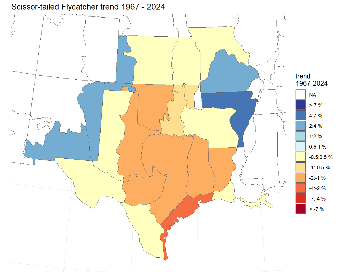
#> # n_obs_sites <int>Trend maps - visualizing the spatial variation in trends
We can plot trend estimates on a map to visualise the spatial patterns in population change.
Barn Swallow example
A model with a suitable number of iterations takes a long time to run (the Barn Swallow model, a species with many counts, years and strata, took 54 hours).
You can download an example of the saved model output for Barn Swallow here:
In this example we’ve placed it in a sub-directory of our working directory called output.
Let’s take a look at the spatial GAMYE model for the Barn Swallow.
First we load the data
BARS <- readRDS("output/Barn_Swallow_gamye_spatial.rds")We can investigate the model meta data
BARS$meta_data
#> $stratify_by
#> [1] "bbs_cws"
#>
#> $stratify_type
#> [1] "standard"
#>
#> $species
#> [1] "Barn Swallow"
#>
#> $model
#> [1] "gamye"
#>
#> $model_variant
#> [1] "spatial"
#>
#> $model_file
#> [1] "C:/Users/SmithAC/AppData/Local/R/win-library/4.2/bbsBayes2/models/gamye_spatial_bbs_CV.stan"
#>
#> $run_date
#> [1] "2023-01-20 13:27:49 EST"
#>
#> $bbsBayes2_version
#> [1] "1.0.0"
#>
#> $cmdstan_path
#> [1] "C:/Users/SmithAC/Documents/.cmdstan/wsl-cmdstan-2.30.1"
#>
#> $cmdstan_version
#> [1] "2.30.1"
See the length of the run in seconds or hours
BARS$model_fit$time()
#> $total
#> [1] 197011.7
#>
#> $chains
#>   chain_id   warmup sampling  total
#> 1        1  82393.1  46100.9 128494
#> 2        2  85907.6 111101.0 197009
#> 3        3 113442.0  54516.1 167958
#> 4        4 113073.0  54597.2 167670
BARS$model_fit$time()$total/3600
#> [1] 54.72546
Now create the indices and trends
BARS_indices <- generate_indices(BARS)
#> Processing region continent
#> Processing region stratum

BARS_index_plots <- plot_indices(BARS_indices,
                                 add_observed_means = TRUE,
                                 add_number_routes = TRUE)

BARS_continent <- BARS_index_plots[["continent"]]
print(BARS_continent)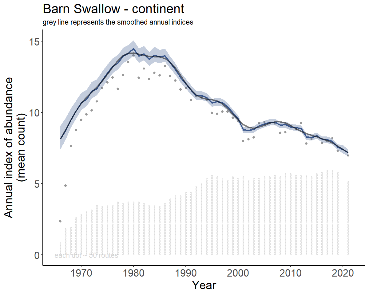
Smoothed population trajectories - gamye model
Above, we’ve plotted the full annual indices (i.e., the population
trajectory) from the gamye model. In the gamye and
slope models, the population trajectory can be decomposed into
two components: the smooth component and the annual fluctuations around
the smooth. The default estimate of the population trajectory uses the
full version of the annual indices
(generate_indices(alternate_n = "n")). For the gamye model
the alternate population trajectory that represents only the
semi-parametric smooth component can be accessed by choosing the
generate_indices(alternate_n = "n_smooth") option. For the
slope model the alternate population trajectory that represents the
linear smooth only can be accessed by choosing the
generate_indices(alternate_n = "n_slope") option. These
smooth trajectories may be useful for trend estimates that vary less
from year-to-year (gamye model) or for an overall linear trend from a
slope model applied to a short time-frame (it’s probably unlikely that a
linear smooth is reasonable for long periods of time).
BARS_smooth_indices <- generate_indices(BARS,
alternate_n = "n_smooth")
#> Processing region continent
#> Processing region stratum
BARS_trends <- generate_trends(BARS_smooth_indices)
BARS_trend_map <- plot_map(BARS_trends)
BARS_trend_map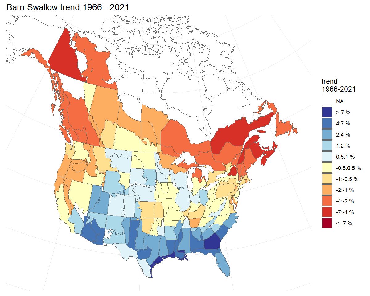 ### Modifying base plots
We can also add the smoothed annual indices to the plots of the full
annual indices from above, taking advantage of the ggplot2 functions such
as geom_line().
library(ggplot2)

smooth_cont_indices <- BARS_smooth_indices$indices %>%
  filter(region == "continent")

BARS_continent_both <- BARS_continent +
  geom_line(data = smooth_cont_indices,
            aes(x = year, y = index),
            alpha = 0.5,
            linewidth = 1)+
  labs(subtitle = "grey line represents the smoothed annual indices")

print(BARS_continent_both)
Check out the other articles to explore more advanced usage or the function reference to see what functions are available and how to use them in greater detail.