Categorizes custom stratification polygons by province or state if possible.
This can be useful for calculating regional indices (generate_indices()) or
trends (generate_trends()) on a custom stratification, or if you want to
create a geofaceted plot (plot_geofacet()).
Arguments
- strata_map
sf data frame. Strata polygons to be categorized.
- min_overlap
Numeric. The minimum proportion of overlap between a stratum polygon and a Province or State. Overlap below this proportion will raise warnings.
- plot
Logical. Whether to plot how polygons were assigned to Provinces or States
- keep_spatial
Logical. Whether the output should be a spatial data frame or not.
See also
Other helper functions:
load_map(),
search_species()
Examples
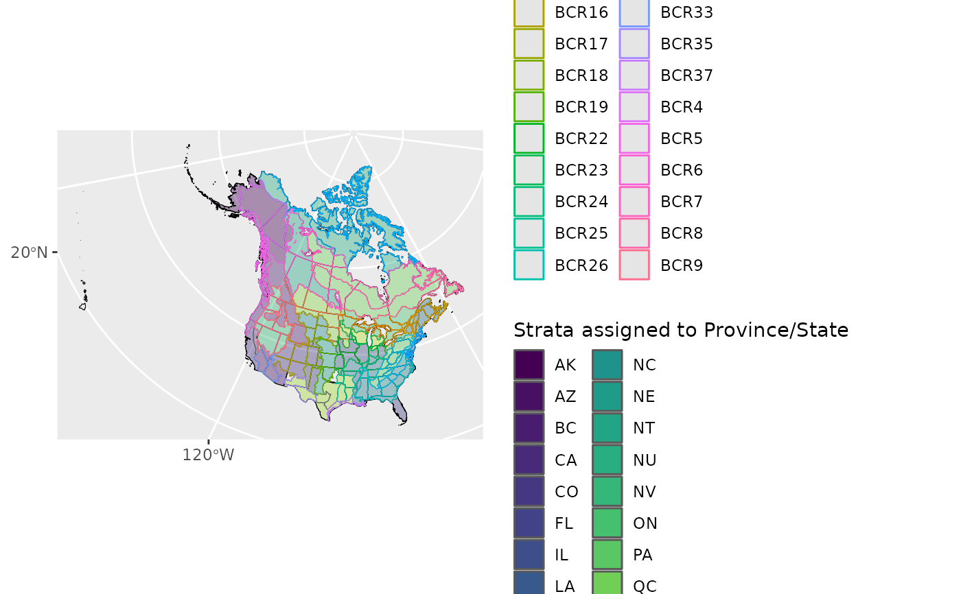
# Demonstration of why we can't divide BCR by Provinces and States!
map <- load_map("bcr")
assign_prov_state(map, plot = TRUE)
#> Warning: 32 strata are assigned to a province or state based on less than the minimum specified overlap

#> Simple feature collection with 227 features and 7 fields
#> Geometry type: GEOMETRY
#> Dimension:     XY
#> Bounding box:  xmin: -5030340 ymin: -1683720 xmax: 2990016 ymax: 4517219
#> Projected CRS: North_America_Albers_Equal_Area_Conic
#> # A tibble: 227 × 8
#>    strata_name prov_state country                  country_code province_state
#>  * <chr>       <chr>      <chr>                    <chr>        <chr>
#>  1 BCR10       BC         United States of America US           Washington
#>  2 BCR5        BC         United States of America US           Washington
#>  3 BCR9        NV         United States of America US           Washington
#>  4 BCR10       BC         Canada                   CA           British Columbia
#>  5 BCR4        AK         Canada                   CA           British Columbia
#>  6 BCR5        BC         Canada                   CA           British Columbia
#>  7 BCR6N       NT         Canada                   CA           British Columbia
#>  8 BCR6S       AB         Canada                   CA           British Columbia
#>  9 BCR9        NV         Canada                   CA           British Columbia
#> 10 BCR10       BC         United States of America US           Idaho
#> # ℹ 217 more rows
#> # ℹ 3 more variables: geom <GEOMETRY [m]>, p_area <dbl>, note <chr>

# Use custom stratification, using sf map object
# e.g. with WBPHS stratum boundaries 2019
# available: https://ecos.fws.gov/ServCat/Reference/Profile/142628

if (FALSE) { # \dontrun{
map <- sf::read_sf("../WBPHS_Stratum_Boundaries_2019") %>%
  rename(strata_name = STRAT) # expects this column
s <- assign_prov_state(map, plot = TRUE)
# Some don't divide nicely, we could try a different min_overlap

s <- assign_prov_state(map, min_overlap = 0.6, plot = TRUE)
} # }
#> Simple feature collection with 227 features and 7 fields
#> Geometry type: GEOMETRY
#> Dimension: XY
#> Bounding box: xmin: -5030340 ymin: -1683720 xmax: 2990016 ymax: 4517219
#> Projected CRS: North_America_Albers_Equal_Area_Conic
#> # A tibble: 227 × 8
#> strata_name prov_state country country_code province_state
#> * <chr> <chr> <chr> <chr> <chr>
#> 1 BCR10 BC United States of America US Washington
#> 2 BCR5 BC United States of America US Washington
#> 3 BCR9 NV United States of America US Washington
#> 4 BCR10 BC Canada CA British Columbia
#> 5 BCR4 AK Canada CA British Columbia
#> 6 BCR5 BC Canada CA British Columbia
#> 7 BCR6N NT Canada CA British Columbia
#> 8 BCR6S AB Canada CA British Columbia
#> 9 BCR9 NV Canada CA British Columbia
#> 10 BCR10 BC United States of America US Idaho
#> # ℹ 217 more rows
#> # ℹ 3 more variables: geom <GEOMETRY [m]>, p_area <dbl>, note <chr>
# Use custom stratification, using sf map object
# e.g. with WBPHS stratum boundaries 2019
# available: https://ecos.fws.gov/ServCat/Reference/Profile/142628
if (FALSE) { # \dontrun{
map <- sf::read_sf("../WBPHS_Stratum_Boundaries_2019") %>%
rename(strata_name = STRAT) # expects this column
s <- assign_prov_state(map, plot = TRUE)
# Some don't divide nicely, we could try a different min_overlap
s <- assign_prov_state(map, min_overlap = 0.6, plot = TRUE)
} # }