Generates the indices plot for each stratum modelled.
Usage
plot_indices(
  indices = NULL,
  ci_width = 0.95,
  min_year = NULL,
  max_year = NULL,
  title = TRUE,
  title_size = 20,
  axis_title_size = 18,
  axis_text_size = 16,
  line_width = 1,
  spaghetti = FALSE,
  n_spaghetti = 100,
  alpha_spaghetti = 0.2,
  add_observed_means = FALSE,
  add_number_routes = FALSE
)
Arguments
- indices
List. Indices generated by
generate_indices().- ci_width
Numeric. Quantile defining the width of the plotted credible interval. Defaults to 0.95 (lower = 0.025 and upper = 0.975). Note these quantiles need to have been precalculated in
generate_indices().- min_year
Numeric. Minimum year to plot.
- max_year
Numeric. Maximum year to plot.
- title
Logical. Whether to include a title on the plot.
- title_size
Numeric. Font size of plot title. Defaults to 20
- axis_title_size
Numeric. Font size of axis titles. Defaults to 18
- axis_text_size
Numeric. Font size of axis text. Defaults to 16
- line_width
Numeric. Size of the trajectory line. Defaults to 1
- spaghetti
Logical. False by default. Plotting option to visualise the uncertainty in the estimated population trajectories. Instead of plotting the trajectory as a single line with an uncertainty bound, if TRUE, then the plot shows a sample of the posterior distribution of the estimated population trajectories. E.g., 100 semi-transparent lines, each representing one posterior draw of the population trajectory.
- n_spaghetti
Integer. 100 by default. Number of posterior draws of the population trajectory to include in the plot. Ignored if spaghetti = FALSE.
- alpha_spaghetti
Numeric between 0 and 1, 0.2 by default. Alpha value - transparency of each individual population trajectory line in the spaghetti plot. Ignored if spaghetti = FALSE.
- add_observed_means
Logical. Whether to include points indicating the observed mean counts. Default
FALSE. Note: scale of observed means and annual indices may not match due to imbalanced sampling among routes. Also, pattern of change in observed means through time should reflect estimated population trajectories for strata-level summaries. However, the temporal patterns may be very different between means and annual indices for composite regions (e.g., continental, state, province, or BCR) because the indices for composite regions account for the variation in area weights and variation in relative abundances among strata, and the observed mean counts do not. For strata-level assessments, these observed means can be a useful model assessment tool. For composite regions, their interpretation is more complicated.- add_number_routes
Logical. Whether to superimpose dotplot showing the number of BBS routes included in each year. This is useful as a visual check on the relative data-density through time because in most cases the number of observations increases over time.
See also
Other indices and trends functions:
generate_indices(),
generate_trends(),
plot_geofacet(),
plot_map()
Examples
# Using the example model for Pacific Wrens...
# Generate country, continent, and stratum indices
i <- generate_indices(model_output = pacific_wren_model,
regions = c("country", "continent", "stratum"))
#> Processing region country
#> Processing region continent
#> Processing region stratum
# Now, plot_indices() will generate a list of plots for all regions
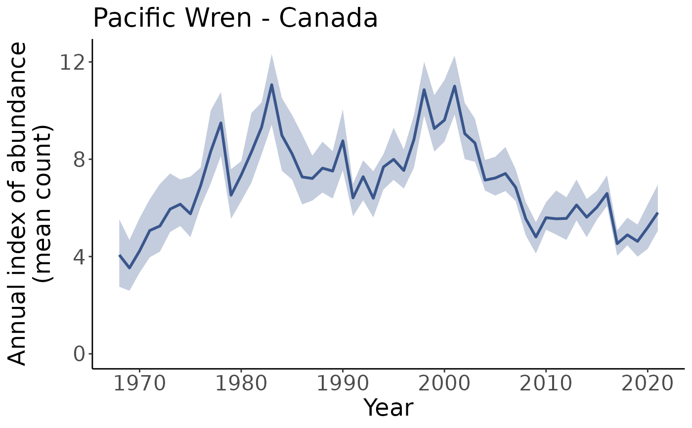
plots <- plot_indices(i)
# To view any plot, use [[i]]
plots[[1]]
 names(plots)
#> [1] "Canada" "United_States_of_America"
#> [3] "continent" "CA_AB_10"
#> [5] "CA_BC_10" "CA_BC_4"
#> [7] "CA_BC_5" "CA_BC_9"
#> [9] "US_AK_2" "US_AK_4"
#> [11] "US_AK_5" "US_CA_15"
#> [13] "US_CA_32" "US_CA_5"
#> [15] "US_ID_10" "US_MT_10"
#> [17] "US_OR_10" "US_OR_5"
#> [19] "US_OR_9" "US_WA_10"
#> [21] "US_WA_5" "US_WA_9"
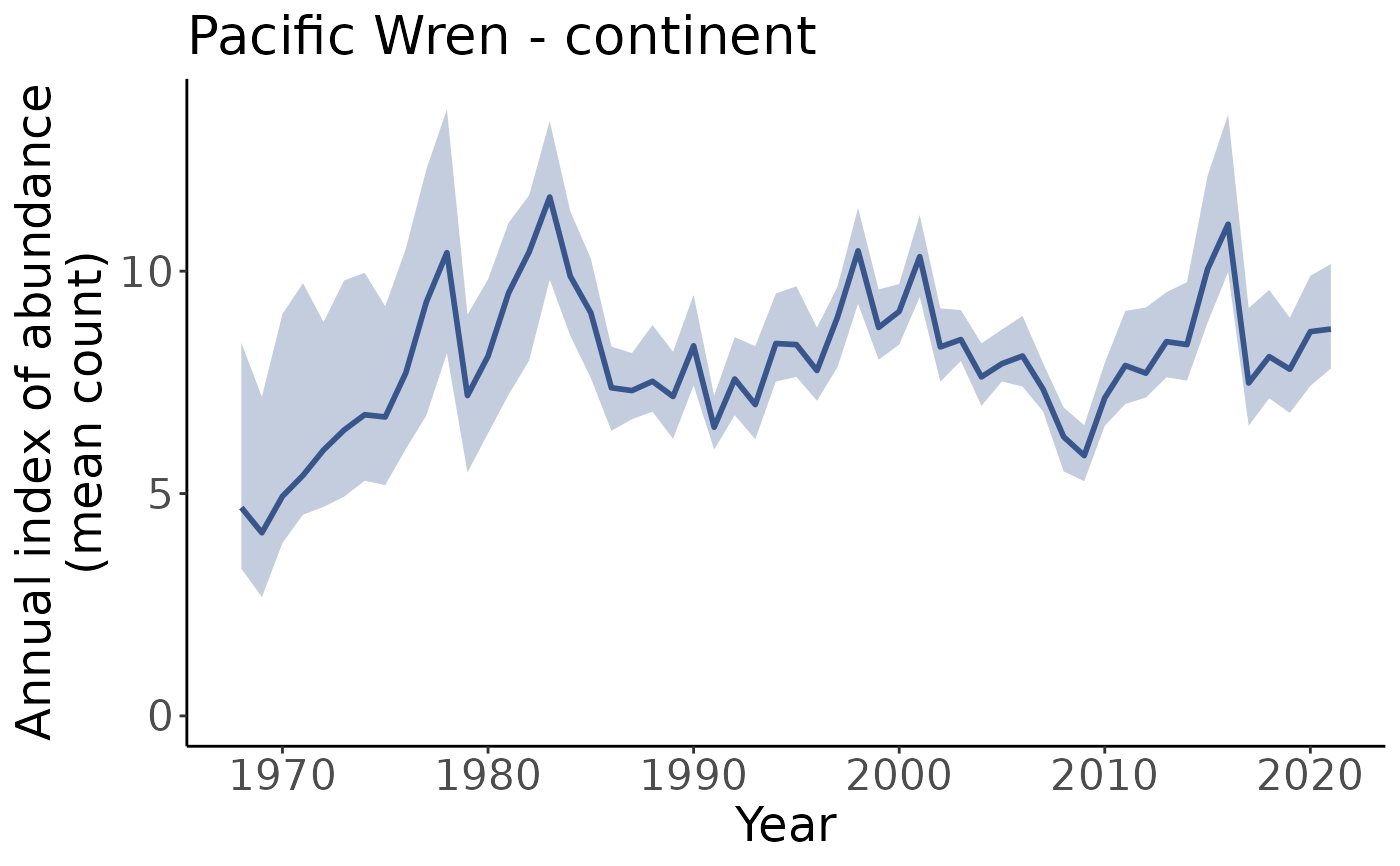
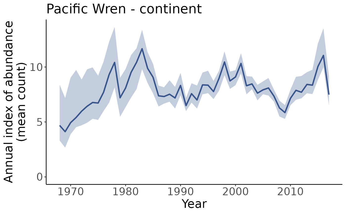
# Suppose we wanted to access the continental plot. We could do so with
plots[["continent"]]
names(plots)
#> [1] "Canada" "United_States_of_America"
#> [3] "continent" "CA_AB_10"
#> [5] "CA_BC_10" "CA_BC_4"
#> [7] "CA_BC_5" "CA_BC_9"
#> [9] "US_AK_2" "US_AK_4"
#> [11] "US_AK_5" "US_CA_15"
#> [13] "US_CA_32" "US_CA_5"
#> [15] "US_ID_10" "US_MT_10"
#> [17] "US_OR_10" "US_OR_5"
#> [19] "US_OR_9" "US_WA_10"
#> [21] "US_WA_5" "US_WA_9"
# Suppose we wanted to access the continental plot. We could do so with
plots[["continent"]]
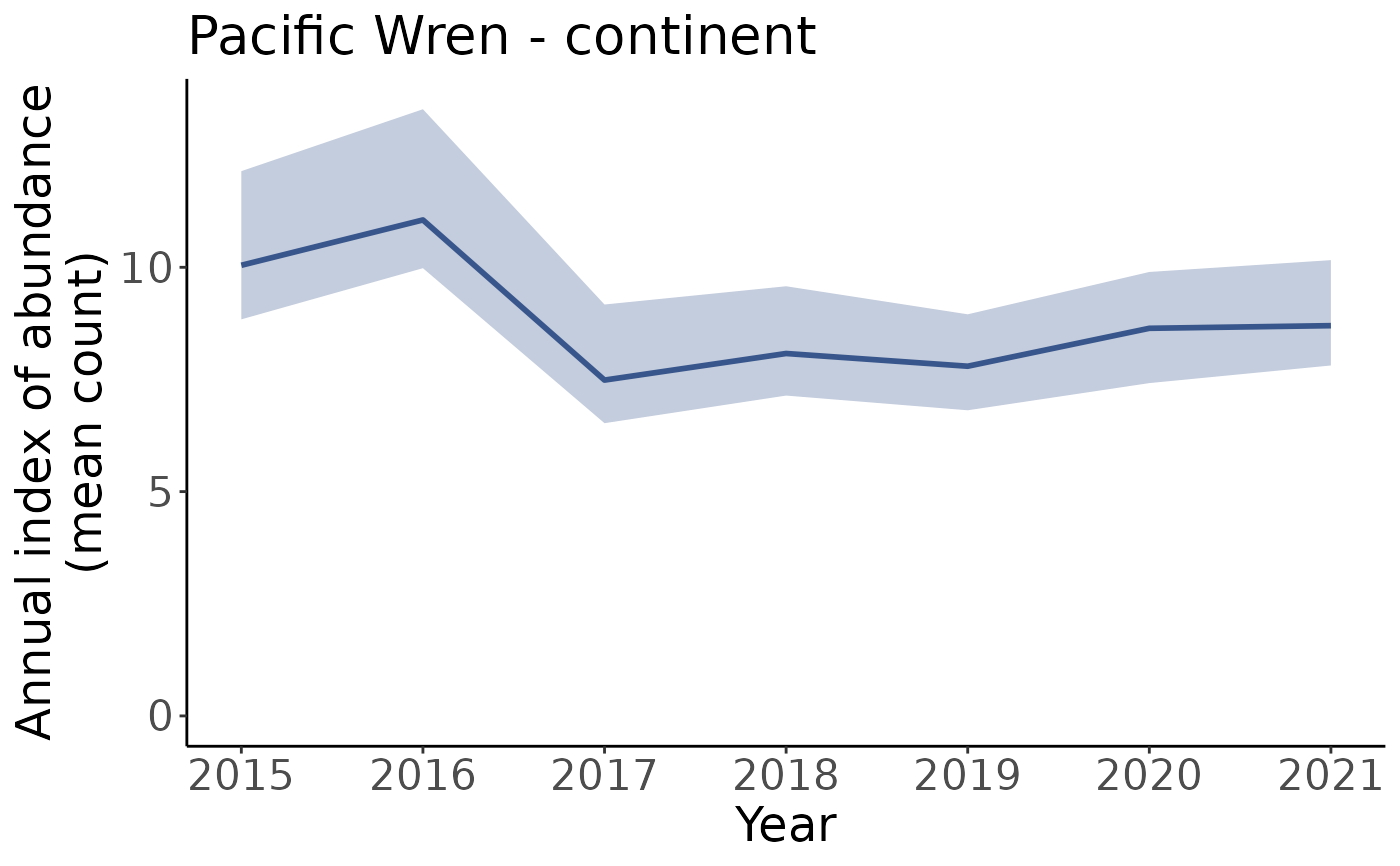
 # You can specify to only plot a subset of years using min_year and max_year
# Plots indices from 2015 onward
p_2015_min <- plot_indices(i, min_year = 2015)
p_2015_min[["continent"]]
# You can specify to only plot a subset of years using min_year and max_year
# Plots indices from 2015 onward
p_2015_min <- plot_indices(i, min_year = 2015)
p_2015_min[["continent"]]
 #Plot up indices up to the year 2017
p_2017_max <- plot_indices(i, max_year = 2017)
p_2017_max[["continent"]]
#Plot up indices up to the year 2017
p_2017_max <- plot_indices(i, max_year = 2017)
p_2017_max[["continent"]]
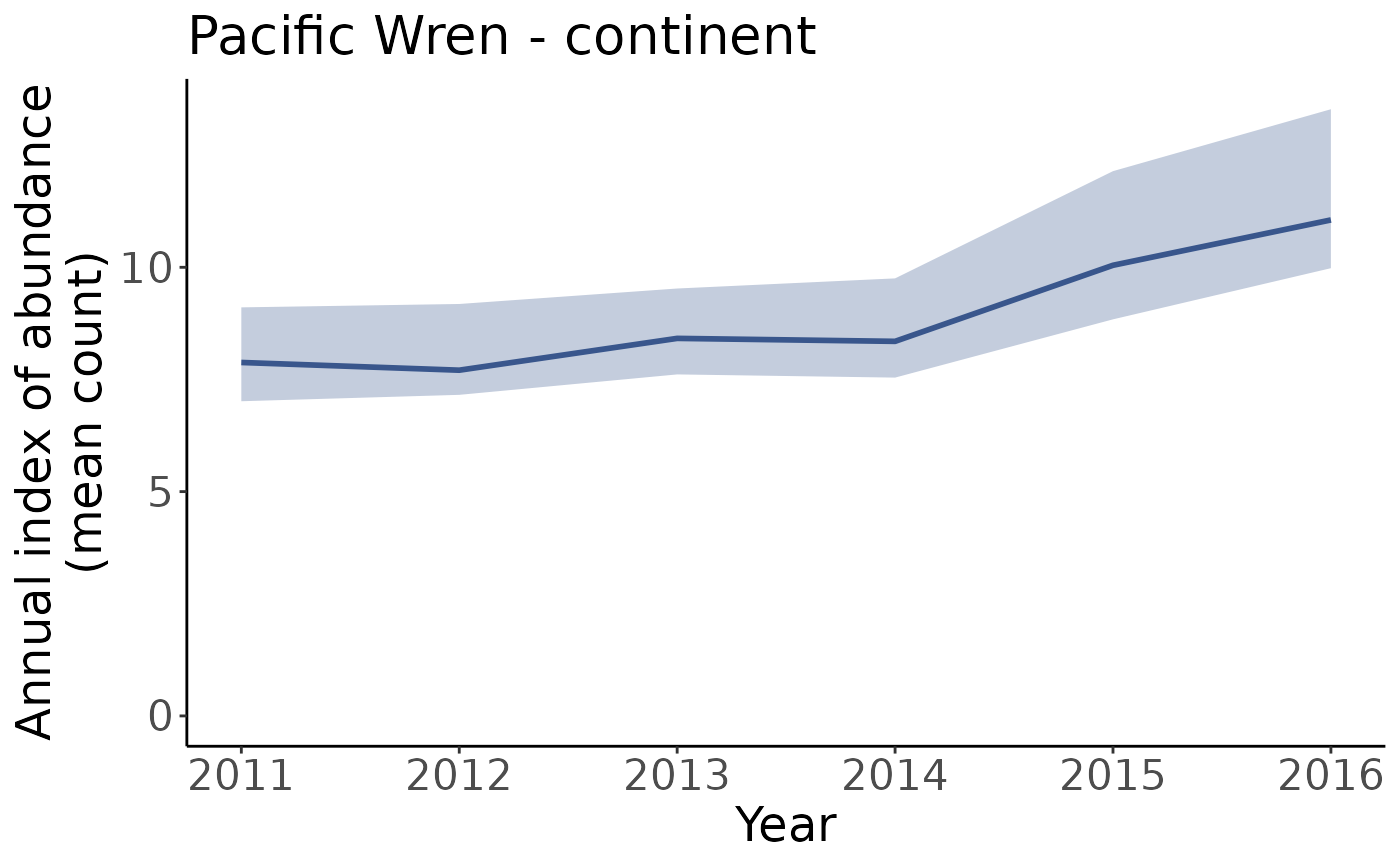
 #Plot indices between 2011 and 2016
p_2011_2016 <- plot_indices(i, min_year = 2011, max_year = 2016)
p_2011_2016[["continent"]]
#Plot indices between 2011 and 2016
p_2011_2016 <- plot_indices(i, min_year = 2011, max_year = 2016)
p_2011_2016[["continent"]]