library(bbsBayes2)
library(sf)       # Spatial data manipulations
library(dplyr)    # General data manipulations
library(ggplot2)  # Plotting
library(patchwork) # mutli-plot
In this vignette we’ll explore the various ways you can stratify the BBS data in preparation for running the models.
You can use existing, pre-defined stratifications, subset an existing stratification (e.g., clip the data to your area of interest), or load your own custom stratification, either using a completely new set of spatial data, or by modifying the spatial polygons of an existing strata.
This vignette assumes that the BBS data have already been downloaded and that you are familiar with the basics of the bbsBayes2 workflow
Stratifying with built-in stratifications
The built-in stratifications are bbs, bbs_usgs, bbs_cws, bcr, bcr_old, latlong, prov_state.
-
bbs– New as of Version 1.1.3.1. Intersections of Political regions X Updated Bird Conservation Regions (Stratification used by the Canadian Wildlife Service [CWS] for national status reporting as of 2024) -
bbs_cws– Intersections of Political regions X Bird Conservation Regions (Stratification formerly used by the Canadian Wildlife Service [CWS] for national status reporting) -
bbs_usgs– Intersections of Political regions X Bird Conservation Regions (Stratification used by the United Status Geological Survey [USGS] for national status reporting) -
bcr– Updated (2025) Bird Conservation Regions, including the subdivisions of four former northern BCRs (3, 6, 7, and 8) into the following 10 BCRs: 3C, 3N, 3S, 6N, 6S, 7E, 7W, 7H, 8E and 8W. -
bcr_old– Bird Conservation Regions used prior to version 1.1.3.1, includes large northern BCRs (3, 6, 7, and 8). Primarily included for reproducibility. -
prov_state– Political regions only - states, provinces, and territories -
latlong– Grid-cells of 1 degree of latitude X 1 degree of longitude, aka “degree-blocks”. These are the original survey design strata for the BBS. Routes are established at randomized locations within these degree-blocks.
You can visualize these stratifications by looking at the maps
included in bbsBayes2 with load_map().
ggplot(data = load_map("bbs"), aes(fill = strata_name)) +
  geom_sf() +
  scale_fill_viridis_d(guide = "none")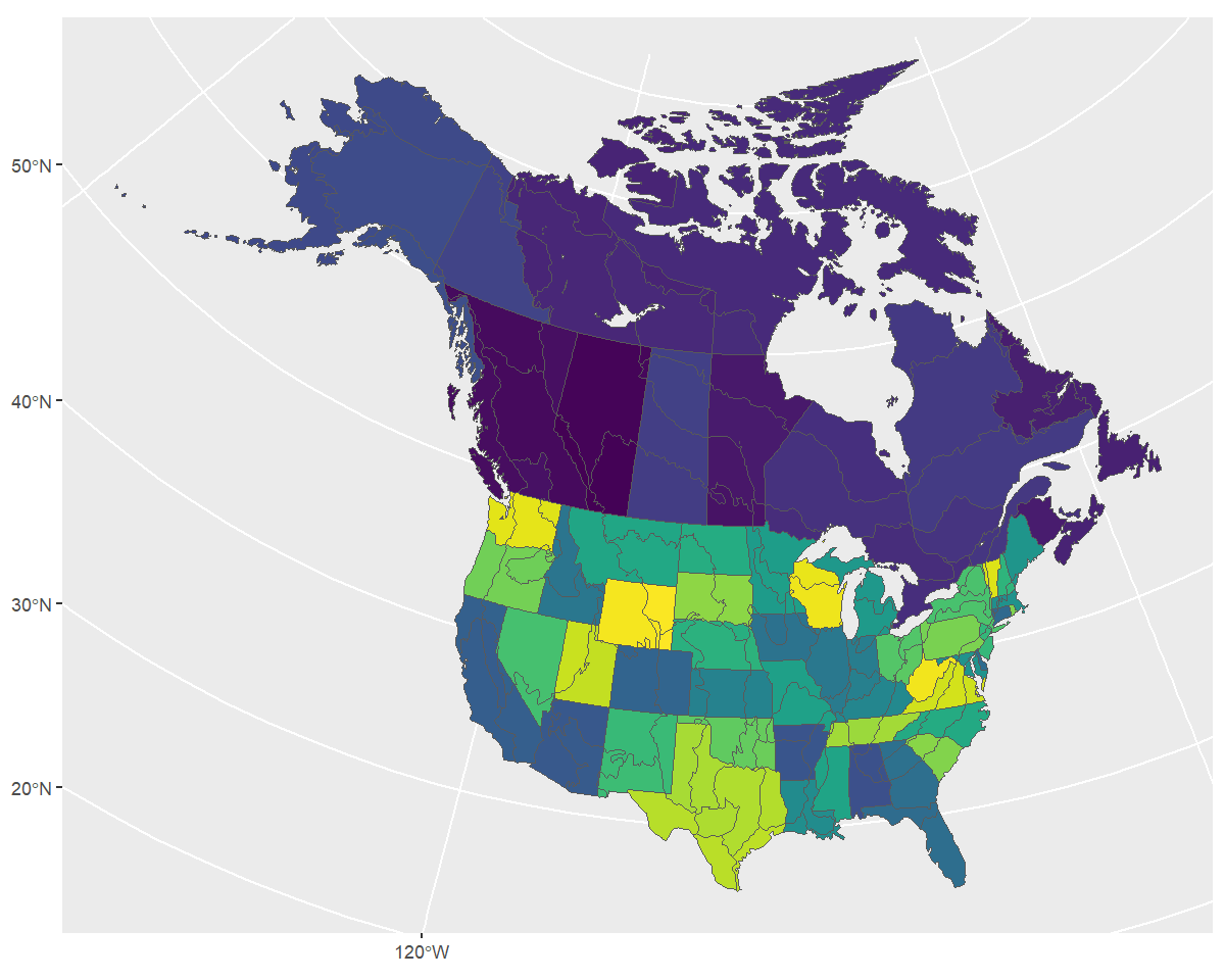
To stratify BBS data, you can use these existing stratifications by
specifying by = "name" in the stratify()
function.
s <- stratify(by = "bbs_usgs", species = "Mallard")
#> Using 'bbs_usgs' (standard) stratification
#> Loading BBS data...
#> Filtering to species Mallard (1320)
#> Stratifying data...
#> Preparing strata (ESRI:102008; North_America_Albers_Equal_Area_Conic)...
#>   Calculating area weights...
#>   Joining routes to spatial layer...
#>   Renaming routes...
#>   Omitting 2,436/127,482 surveys, on 111 unique routes that do not match a stratum.
#>     To see omitted routes use `return_omitted = TRUE` (see ?stratify)
The latlong stratification - special note
The latlong stratification by = "latlong" is the
finest-scale stratification built into the package, and so it divides
the BBS data into many more strata-units than other stratifications.
Therefore, you may wish to adjust the minimum data inclusion criteria
when preparing the data. Specifically, setting
min_n_routes = 1 ensures that every grid-cell with at least
one BBS route can be included. There are many degree-blocks that have
only one route, as this is the original sampling design goal of the BBS
(at least one route within each degree-block).
s <- stratify(by = "latlong", species = "Mallard", use_map = FALSE)
#> Using 'latlong' (standard) stratification
#> Loading BBS data...
#> Filtering to species Mallard (1320)
#> Stratifying data...
#>   Renaming routes...
#>   Omitting 115/127,482 surveys, on 7 unique routes that do not match a stratum.
#>     To see omitted routes use `return_omitted = TRUE` (see ?stratify)
p <- prepare_data(s, min_n_routes = 1)
Custom stratifications
bbsBayes2 can stratify the BBS data using any polygon map as input.
Load a custom stratification map
To define a completely different stratification, you’ll need to provide a spatial data object with polygons defining your strata.
In our example we’ll use WBPHS stratum boundaries. This is available from available from the US Fish and Wildlife Service Catalogue: https://ecos.fws.gov/ServCat/Reference/Profile/142628
To run this locally, download the file manually and unzip the shapefile contents into subdirectory of your working directory called output.
To use this file in bbsBayes2, we need to load it as an sf object using the sf package.
map <- sf::read_sf("output/WBPHS_stratum_boundaries.shp")
ggplot(map, aes(fill = factor(stratum))) +
geom_sf() +
scale_fill_viridis_d(guide = "none")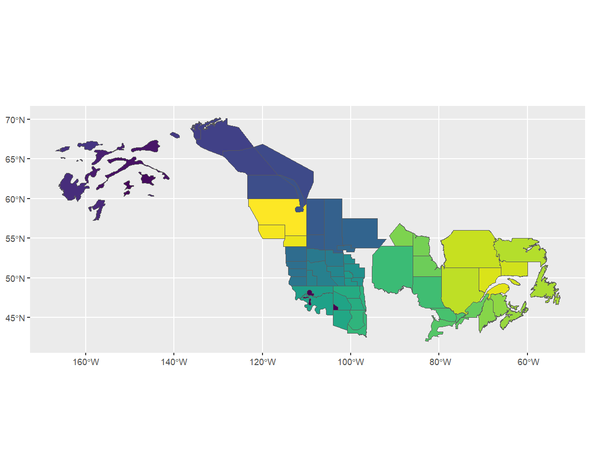 ### Identify the strata names
We see that it has one column that reflects the stratum names. First
we’ll rename this column to strata_name, and mutate it into
a character value, so that the stratify() function knows
what attribute includes the names that define each stratum.
map <- rename(map, strata_name = stratum) %>%
        mutate(strata_name = as.character(strata_name))
Stratify the data
Now we have the spatial data and relevant information to pass to
stratify().
When using a custom stratification, the by argument is
just a user-defined arbitrary name to document which stratification was
used. This name gets passed into the meta data of the following steps
and the final fitted model. Let’s use something informative, but short
(although there’s no limit). We also need to give the function our
map.
s <- stratify(by = "WBPHS", species = "Mallard", strata_custom = map)
#> Using 'wbphs' (custom) stratification
#> Loading BBS data...
#> Filtering to species Mallard (1320)
#> Stratifying data...
#> Preparing strata (EPSG:4326; WGS 84)...
#>   Summarizing strata...
#>   Calculating area weights...
#>   Joining routes to spatial layer...
#>   Renaming routes...
#>   Omitting 106,608/127,482 surveys, on 3,783 unique routes that do not match a stratum.
#>     To see omitted routes use `return_omitted = TRUE` (see ?stratify)
Note that strata names are automatically put into lower case for consistency.
We can take a quick look at the output, by looking at the meta data and routes contained therein.
s[["meta_data"]]
#> $stratify_by
#> [1] "wbphs"
#>
#> $stratify_type
#> [1] "custom"
#>
#> $species
#> [1] "Mallard"
#>
#> $sp_aou
#> [1] 1320

s[["routes_strata"]]
#> # A tibble: 20,874 × 34
#>    strata_name country_num state_num route route_name active   bcr route_type_id route_type_detail_id
#>    <chr>             <dbl>     <dbl> <chr> <chr>       <dbl> <dbl>         <dbl>                <dbl>
#>  1 3                   840         3 3-4   BIRCH LAKE      1     4             1                    1
#>  2 3                   840         3 3-4   BIRCH LAKE      1     4             1                    1
#>  3 3                   840         3 3-4   BIRCH LAKE      1     4             1                    1
#>  4 3                   840         3 3-4   BIRCH LAKE      1     4             1                    1
#>  5 3                   840         3 3-4   BIRCH LAKE      1     4             1                    1
#>  6 3                   840         3 3-4   BIRCH LAKE      1     4             1                    1
#>  7 3                   840         3 3-4   BIRCH LAKE      1     4             1                    1
#>  8 3                   840         3 3-4   BIRCH LAKE      1     4             1                    1
#>  9 3                   840         3 3-4   BIRCH LAKE      1     4             1                    1
#> 10 3                   840         3 3-4   BIRCH LAKE      1     4             1                    1
#> # ℹ 20,864 more rows
#> # ℹ 25 more variables: route_data_id <dbl>, rpid <dbl>, year <dbl>, month <dbl>, day <dbl>, obs_n <dbl>,
#> #   total_spp <dbl>, start_temp <dbl>, end_temp <dbl>, temp_scale <chr>, start_wind <dbl>, end_wind <dbl>,
#> #   start_sky <dbl>, end_sky <dbl>, start_time <dbl>, end_time <dbl>, assistant <dbl>, quality_current_id <dbl>,
#> #   run_type <dbl>, state <chr>, st_abrev <chr>, country <chr>, longitude <dbl>, latitude <dbl>,
#> #   area_sq_km <dbl>
Visualise the new strata and data
To get a different look we can also plot this data on top of our map
using ggplot2. Note that we use factor() to ensure the
strata names are categorical.
rts <- s[["routes_strata"]] %>%
  st_as_sf(coords = c("longitude", "latitude"), crs = 4326)

ggplot() +
  geom_sf(data = map, aes(fill = factor(strata_name)), alpha = 0.3) +
  geom_sf(data = rts, aes(colour = factor(strata_name)), size = 1) +
  scale_fill_viridis_d(aesthetics = c("colour", "fill"), guide = "none")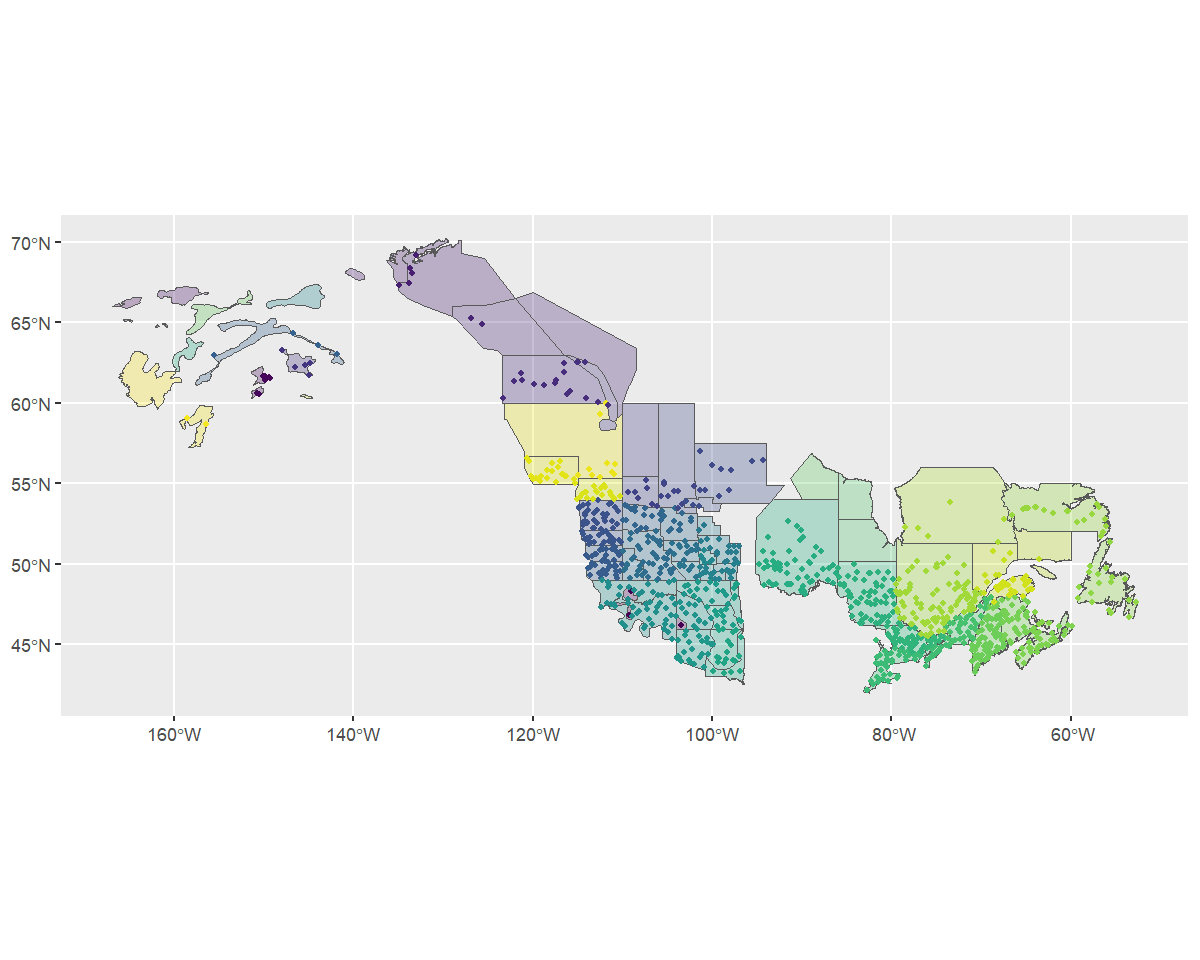
Omitted BBS routes
Based on the message we received during stratification
(Omitting...) and this map, it looks as if our custom
stratification is excluding some BBS data (i.e., routes with starting
locations that are not overlapped by the strata map). This makes sense
because the WBPHS survey area is much smaller than the region covered by
the BBS. However, let’s confirm that the excluded routes are the ones we
expect.
We can re-run the stratification with
return_omitted = TRUE which will attach a data frame of
omitted strata to the output.
s <- stratify(by = "WBPHS", species = "Mallard", strata_custom = map,
              return_omitted = TRUE)
#> Using 'wbphs' (custom) stratification
#> Loading BBS data...
#> Filtering to species Mallard (1320)
#> Stratifying data...
#> Preparing strata (EPSG:4326; WGS 84)...
#>   Summarizing strata...
#>   Calculating area weights...
#>   Joining routes to spatial layer...
#>   Renaming routes...
#>   Omitting 106,608/127,482 surveys, on 3,783 unique routes that do not match a stratum.
#>     Returning omitted routes.
s[["routes_omitted"]]
#> # A tibble: 106,608 × 11
#>     year strata_name country state   route route_name latitude longitude   bcr   obs_n total_spp
#>    <dbl> <chr>       <chr>   <chr>   <chr> <chr>         <dbl>     <dbl> <dbl>   <dbl>     <dbl>
#>  1  1967 <NA>        US      ALABAMA 2-1   ST FLORIAN     34.9     -87.6    27 1140018        56
#>  2  1969 <NA>        US      ALABAMA 2-1   ST FLORIAN     34.9     -87.6    27  990062        52
#>  3  1970 <NA>        US      ALABAMA 2-1   ST FLORIAN     34.9     -87.6    27  990062        52
#>  4  1971 <NA>        US      ALABAMA 2-1   ST FLORIAN     34.9     -87.6    27  990062        56
#>  5  1972 <NA>        US      ALABAMA 2-1   ST FLORIAN     34.9     -87.6    27  990062        54
#>  6  1973 <NA>        US      ALABAMA 2-1   ST FLORIAN     34.9     -87.6    27 1060057        52
#>  7  1974 <NA>        US      ALABAMA 2-1   ST FLORIAN     34.9     -87.6    27 1060057        55
#>  8  1975 <NA>        US      ALABAMA 2-1   ST FLORIAN     34.9     -87.6    27 1060057        59
#>  9  1976 <NA>        US      ALABAMA 2-1   ST FLORIAN     34.9     -87.6    27 1060057        56
#> 10  1977 <NA>        US      ALABAMA 2-1   ST FLORIAN     34.9     -87.6    27 1060057        51
#> # ℹ 106,598 more rows
Let’s take a look.
omitted <- st_as_sf(s[["routes_omitted"]], coords = c("longitude", "latitude"),
                    crs= 4326)

ggplot() +
  geom_sf(data = map, aes(fill = factor(strata_name)), alpha = 0.3) +
  geom_sf(data = rts, aes(colour = factor(strata_name)), size = 1, alpha = 0.5) +
  geom_sf(data = omitted, size = 0.75, alpha = 0.5) +
  scale_fill_viridis_d(aesthetics = c("colour", "fill"), guide = "none")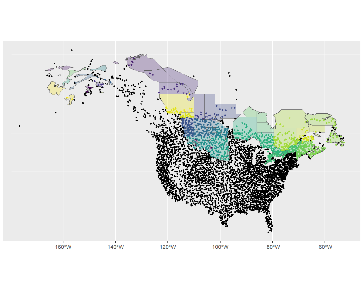
The map shows that most of the omitted routes are routes that are clearly outside of our desired stratification. However, it also shows that there are some BBS route start-points that are just outside of the strata (e.g., some routes in Nova Scotia and Alaska). The user can decide what to do with these sorts of minor overlap issues. For example, buffering the original stratification map might make sense in some situations. For now, we will trust our custom strata map and retain only the BBS routes with start locations inside our strata polygons.
Fitting the model
To fit the model, we follow the standard workflow using our stratified data.
p <- prepare_data(s,
                  min_year = 2000,
                  max_year = 2021) #subset a shorter time-span to speed model-fit
sp <- prepare_spatial(p,map)
#> Preparing spatial data...
#> Supplied strata_map is in a geographic projection. Transforming coordinate reference system to a projected and equal area crs to facilitate mapping and neighbourhood relationships. This will not affect the relationship between strata and the BBS data, only ensures that neighbours are consistently defined and easily mapped.
#>     Summarizing polygons by strata...
#> Identifying neighbours (non-Voronoi method)...
#> Linking islands (isolated groups of nodes)...
#>     Islands found (5). Linking by distance between centroids...
#>     Islands found (4). Linking by distance between centroids...
#>     Islands found (3). Linking by distance between centroids...
#>     Islands found (2). Linking by distance between centroids...
#>     Islands found (1). Linking by distance between centroids...
#> Formating neighbourhood matrices...
#> Plotting neighbourhood matrices...
mp <- prepare_model(sp,model = "first_diff",
                   model_variant = "spatial")
m <- run_model(mp,
               iter_warmup = 500,
               iter_sampling = 100)
Predictions from the model using the custom stratification
Now we can start to look at the indices and trends related to our model.
We can apply the generate_indices() and
generate_trends() functions to the output from our model,
the same as we would with the built-in stratifications.
i <- generate_indices(m)
#> Processing region continent
#> Processing region stratum

t <- generate_trends(i)
And with one additional argument, we can also use the
plot_map() function.
trend_map <- plot_map(t, strata_custom = map)
trend_map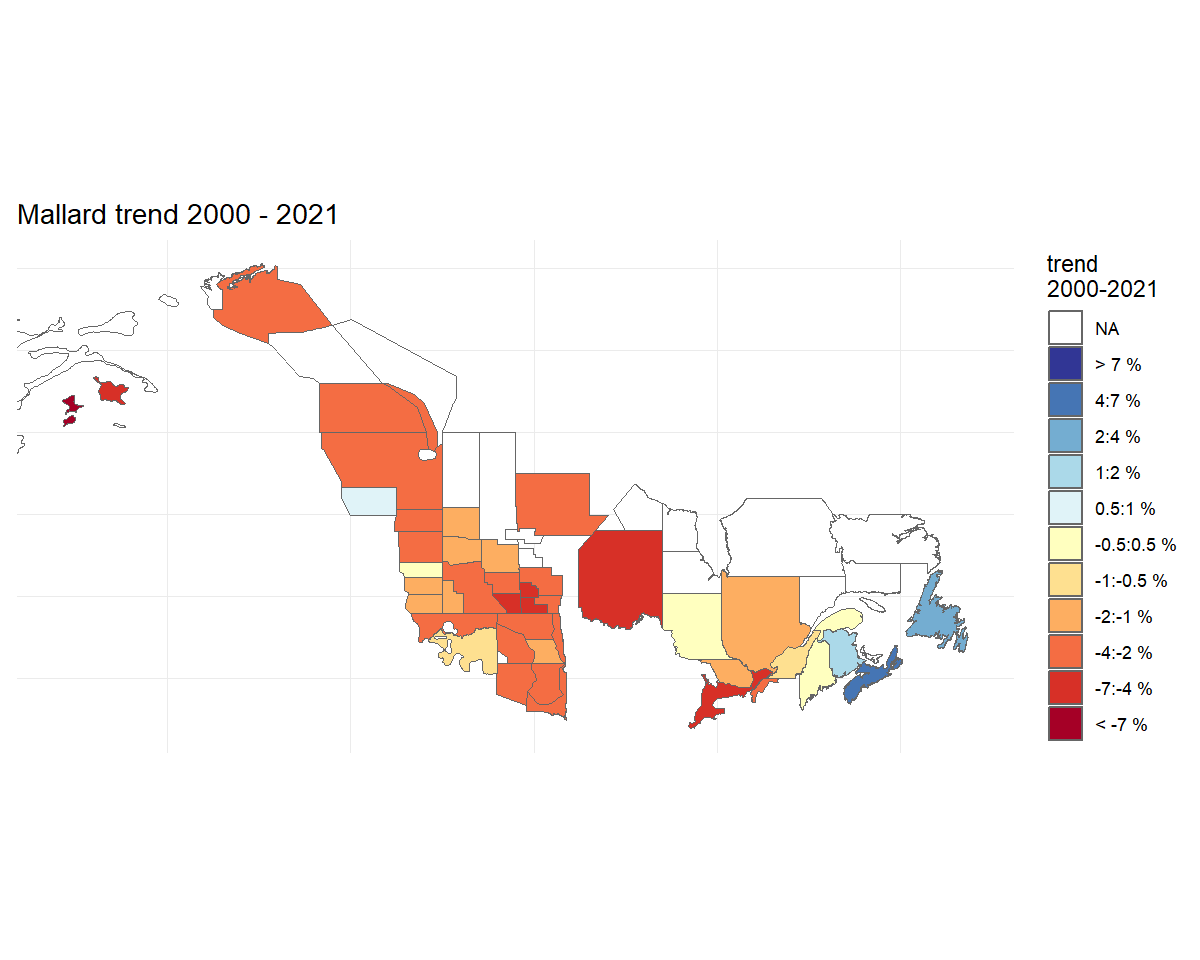
Generating state and province predictions from a custom stratification
A useful feature of the hierarchical Bayesian models for the BBS is the ability to generate formal estimates of indices (annual relative abundance) and trends (rates of population change) for any composite region. Formal estimates meaning we can estimate the full posterior distribution, including a point estimate and its associated uncertainty (credible limits). These composite regions can be defined based on any combination of the underlying strata used to fit the model. For example, using any custom stratification, we can generate estimates for political jurisdictions (countries, states, provinces), as long as we can comfortably designate each of the strata to one of these jurisdictions.
By default, generate_indices() creates indices at two
levels “continent” (the combination of all strata used in the analysis)
and “stratum” (estimates for individual strata). For the two
bbs stratifications (“bbs_usgs” and “bbs_cws”), we can also add
“prov_state”, “bcr”, “bcr_by_country” (where appropriate). For any
custom stratification, we can also add the political jurisdictions
and/or create our own regional divisions and provide them as a
regions_index data frame.
For example, let’s imagine we would like to calculate regional indices for each stratum, country, province/state, as well as for a custom division of eastern and western regions.
First we’ll need to tell the function which strata belong to which province or state, and then which belong to the ‘east’ and which to the ’west.
We’ll start by using a helper function
assign_prov_state(). This function takes a map of strata
and assigns each strata to a province or state depending on the amount
of overlap. By default it will warn if the amount of overlap is less
than 75%, but in this case, we will lower that cutoff to 60%. The plot
gives us a chance to make a quick assessment of whether we’re happy with
how the various strata have been assigned.
rindex <- assign_prov_state(map, min_overlap = 0.6, plot = TRUE)
#> Ignoring unknown labels:
#> • colour : "Less than min_overlap with Province/State"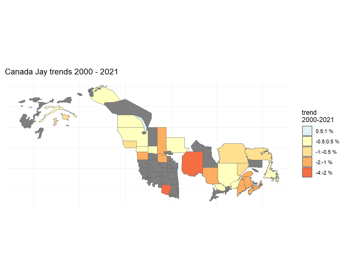
Next we’ll define the east/west divide by hand. If we plot the strata by name, we can pick out which are eastern and which western.
ggplot(rindex) +
  geom_sf(data = load_map(type = "North America")) +
  geom_sf() +
  geom_sf_text(aes(label = strata_name), size = 2)
#> Warning in st_point_on_surface.sfc(sf::st_zm(x)): st_point_on_surface may not give correct results for
#> longitude/latitude data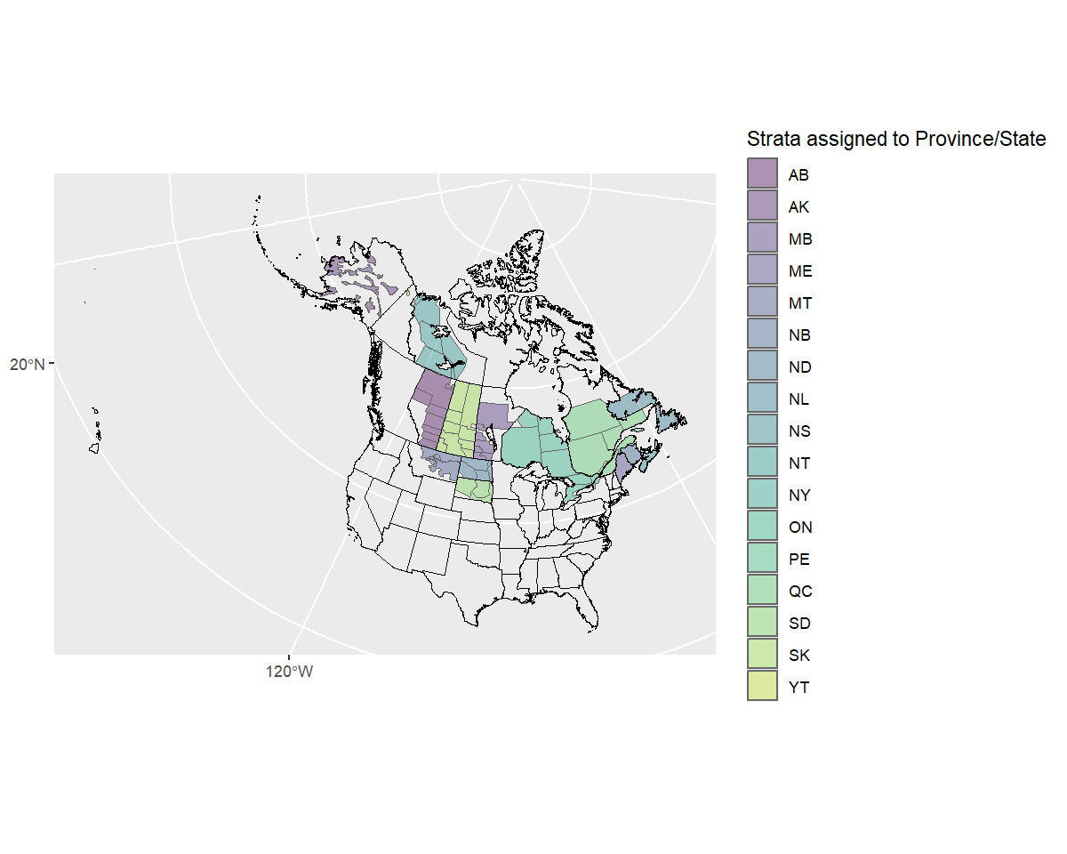
The western and eastern strata seem to be split numerically, such
that the western strata have numbers lower than 50 or greater than 74,
eastern strata have numbers in between. So we’ll add a column to the
rindex dataframe with “east” and “west” character names to
group the strata.
rindex <- mutate(
  rindex,
  east_west = if_else(as.numeric(strata_name) < 50 | as.numeric(strata_name) > 74,
                      "west",
                      "east"))
And now double check that we correctly grouped the strata!
ggplot(data = rindex) +
  geom_sf(data = load_map(type = "North America")) +
  geom_sf(data = rindex, aes(fill = east_west), alpha = 0.5)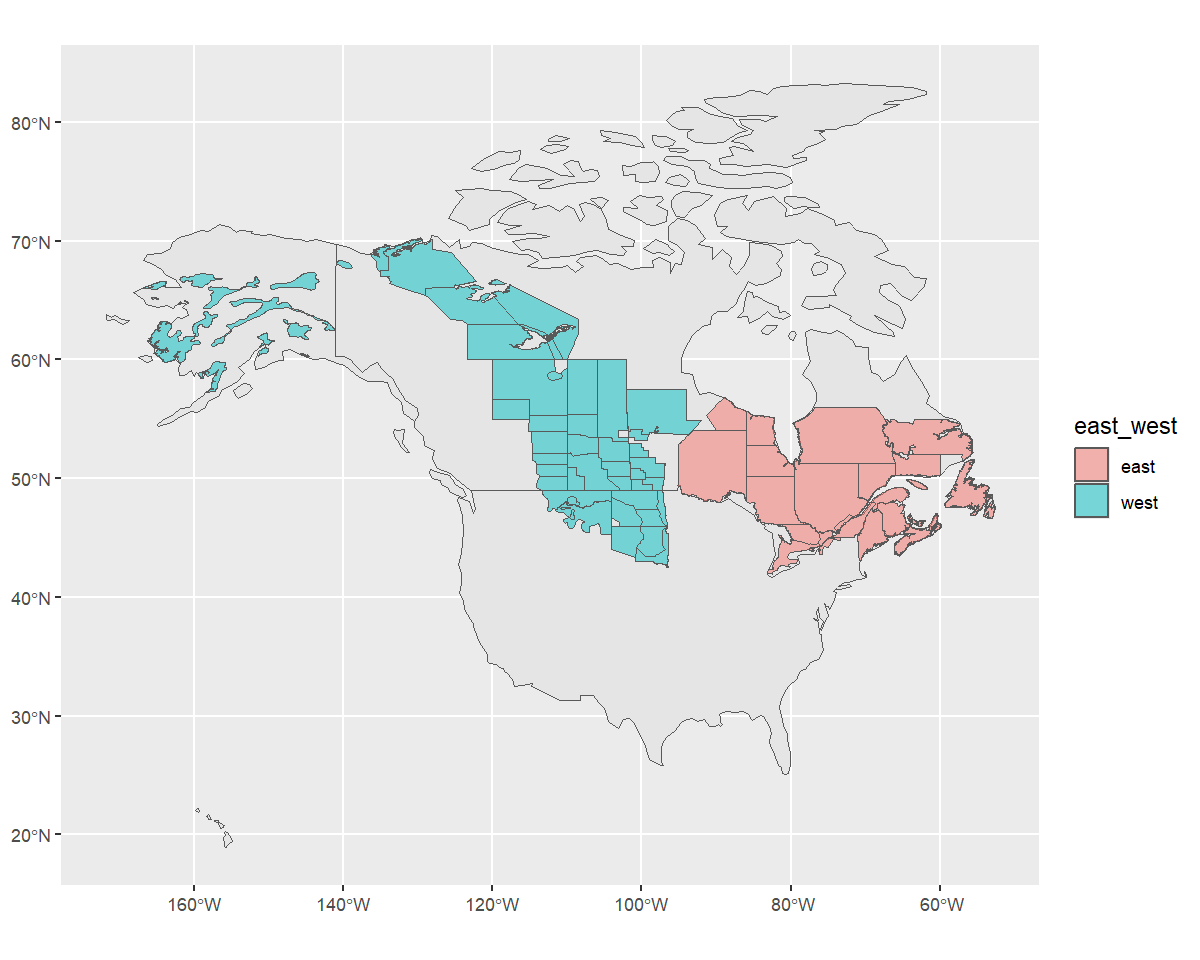
Then supply the rindex object to the
regions_index argument of the
generate_indices() function and include the relevant column
names from the object as regions.
i <- generate_indices(
  m,
  regions = c("stratum", "country", "prov_state", "east_west"),
  regions_index = rindex)
#> Processing region stratum
#> Processing region country
#> Processing region prov_state
#> Processing region east_west

t <- generate_trends(i)
We can plot the population trajectories for each of these regions
with plot_indices().
p <- plot_indices(i)
names(p)
#>  [1] "1"                        "14"                       "17"                       "18"
#>  [5] "2"                        "22"                       "24"                       "26"
#>  [9] "27"                       "28"                       "29"                       "30"
#> [13] "31"                       "32"                       "33"                       "34"
#> [17] "35"                       "37"                       "38"                       "39"
#> [21] "40"                       "41"                       "42"                       "43"
#> [25] "44"                       "45"                       "46"                       "47"
#> [29] "48"                       "49"                       "50"                       "51"
#> [33] "52"                       "53"                       "54"                       "55"
#> [37] "56"                       "62"                       "63"                       "64"
#> [41] "66"                       "68"                       "72"                       "75"
#> [45] "76"                       "77"                       "Canada"                   "United_States_of_America"
#> [49] "AB"                       "AK"                       "MB"                       "ME"
#> [53] "MT"                       "NB"                       "ND"                       "NL"
#> [57] "NS"                       "NT"                       "NY"                       "ON"
#> [61] "QC"                       "SD"                       "SK"                       "east"
#> [65] "west"

p[["east"]] + p[["west"]]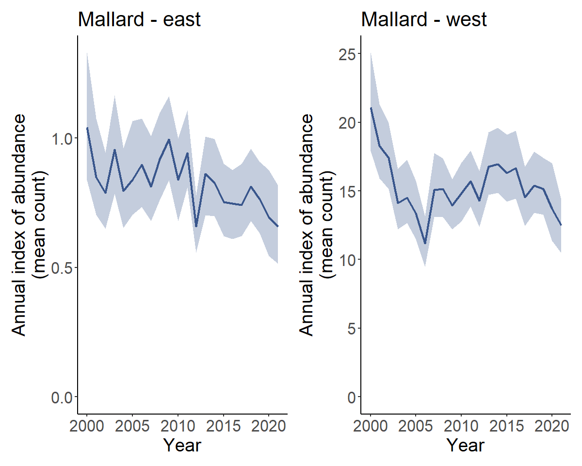
Finally we can even create geofaceted plots (which is only possible in our case because we assigned our strata to Provinces and States and calculated indices for these regions). These geofacet plots can be useful for visualizing the population trajectories of species with broad ranges across many states and provinces.
plot_geofacet(i, trends = t, multiple = TRUE)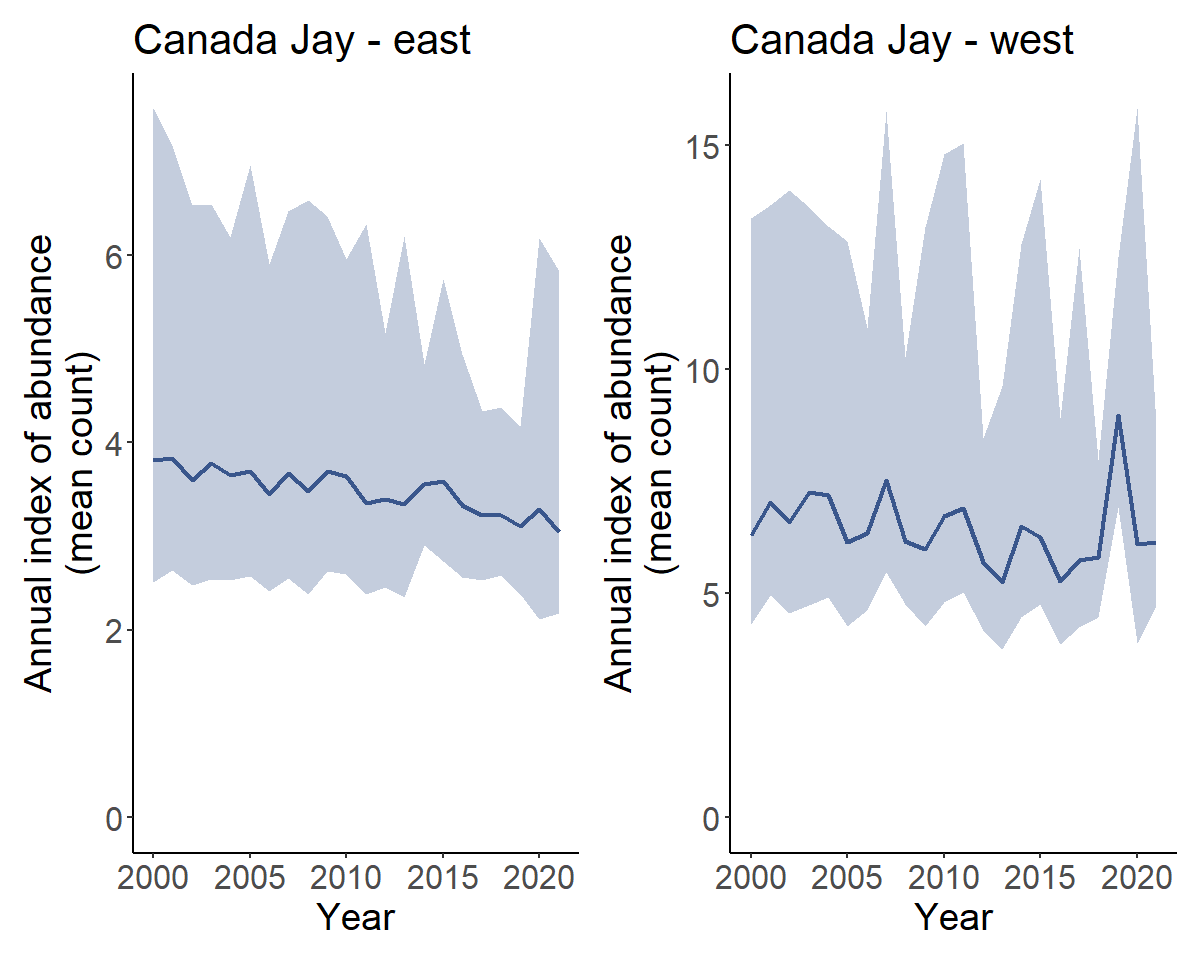
Subsetting an existing stratification
In general, it is often useful to use all of the data for a given species, even if you’re only interested in trends for a portion of the species’ range (estimates of observer effects are informed by all of the data in the analysis). However, there may be situations where the focus of your study is limited to a particular region. For example what if you want to use one of the standard stratifications, but you only want the analysis to be influenced by data from one region, say only Canadian data?
In this case you can subset the BBS CWS stratification to only
Canadian regions, and use that subset of regions as a custom
stratification in the stratify() function.
In addition to maps, stratifications are available as data frames in
the bbs_strata object.
names(bbs_strata)
#> [1] "bbs"        "bbs_usgs"   "bbs_cws"    "bcr"        "bcr_old"    "latlong"    "prov_state"
head(bbs_strata[["bbs_cws"]])
#> # A tibble: 6 × 7
#>   strata_name area_sq_km country country_code prov_state   bcr bcr_by_country
#>   <chr>            <dbl> <chr>   <chr>        <chr>      <dbl> <chr>
#> 1 CA-AB-10        52565. Canada  CA           AB            10 Canada-BCR_10
#> 2 CA-AB-11       149352. Canada  CA           AB            11 Canada-BCR_11
#> 3 CA-AB-6        445135. Canada  CA           AB             6 Canada-BCR_6
#> 4 CA-AB-8          6987. Canada  CA           AB             8 Canada-BCR_8
#> 5 CA-BC-10       383006. Canada  CA           BC            10 Canada-BCR_10
#> 6 CA-BC-4        193180. Canada  CA           BC             4 Canada-BCR_4
We can now modify and use this data frame as we like.
my_cws <- filter(bbs_strata[["bbs_cws"]], country == "Canada")
s <- stratify(by = "bbs_cws", species = "Mallard", strata_custom = my_cws)
#> Using 'bbs_cws' (subset) stratification
#> Loading BBS data...
#> Filtering to species Mallard (1320)
#> Stratifying data...
#> Preparing strata (ESRI:102008; North_America_Albers_Equal_Area_Conic)...
#>   Calculating area weights...
#>   Joining routes to spatial layer...
#>   Renaming routes...
#>   Omitting 2,436/127,482 surveys, on 111 unique routes that do not match a stratum.
#>     To see omitted routes use `return_omitted = TRUE` (see ?stratify)
Note that the stratification is now “bbs_cws” and “subset”
s[["meta_data"]]
#> $stratify_by
#> [1] "bbs_cws"
#>
#> $stratify_type
#> [1] "subset"
#>
#> $species
#> [1] "Mallard"
#>
#> $sp_aou
#> [1] 1320
We can see the strata included by looking at the
meta_strata
print(s[["meta_strata"]], n = Inf)
#> # A tibble: 184 × 7
#> strata_name area_sq_km country country_code prov_state bcr bcr_by_country
#> <chr> <dbl> <chr> <chr> <chr> <dbl> <chr>
#> 1 CA-AB-10 52565. Canada CA AB 10 Canada-BCR_10
#> 2 CA-AB-11 149352. Canada CA AB 11 Canada-BCR_11
#> 3 CA-AB-6 445135. Canada CA AB 6 Canada-BCR_6
#> 4 CA-BC-10 383006. Canada CA BC 10 Canada-BCR_10
#> 5 CA-BC-4 193180. Canada CA BC 4 Canada-BCR_4
#> 6 CA-BC-5 199820. Canada CA BC 5 Canada-BCR_5
#> 7 CA-BC-6 106917. Canada CA BC 6 Canada-BCR_6
#> 8 CA-BC-9 59939. Canada CA BC 9 Canada-BCR_9
#> 9 CA-BCR7-7 1743744. Canada CA BCR7 7 Canada-BCR_7
#> 10 CA-MB-11 70101. Canada CA MB 11 Canada-BCR_11
#> 11 CA-MB-12 15312. Canada CA MB 12 Canada-BCR_12
#> 12 CA-MB-6 127190. Canada CA MB 6 Canada-BCR_6
#> 13 CA-MB-8 234151. Canada CA MB 8 Canada-BCR_8
#> 14 CA-NB-14 72991. Canada CA NB 14 Canada-BCR_14
#> 15 CA-NL-8 157083. Canada CA NL 8 Canada-BCR_8
#> 16 CA-NSPE-14 61502. Canada CA NSPE 14 Canada-BCR_14
#> 17 CA-NT-3 394769. Canada CA NT 3 Canada-BCR_3
#> 18 CA-NT-6 509423. Canada CA NT 6 Canada-BCR_6
#> 19 CA-NU-3 1969549. Canada CA NU 3 Canada-BCR_3
#> 20 CA-ON-12 206181. Canada CA ON 12 Canada-BCR_12
#> 21 CA-ON-13 83859. Canada CA ON 13 Canada-BCR_13
#> 22 CA-ON-8 435545. Canada CA ON 8 Canada-BCR_8
#> 23 CA-QC-12 174314. Canada CA QC 12 Canada-BCR_12
#> 24 CA-QC-13 28409. Canada CA QC 13 Canada-BCR_13
#> 25 CA-QC-14 67711. Canada CA QC 14 Canada-BCR_14
#> 26 CA-QC-8 470310. Canada CA QC 8 Canada-BCR_8
#> 27 CA-SK-11 241315. Canada CA SK 11 Canada-BCR_11
#> 28 CA-SK-6 177763. Canada CA SK 6 Canada-BCR_6
#> 29 CA-SK-8 188615. Canada CA SK 8 Canada-BCR_8
#> 30 CA-YT-4 435349. Canada CA YT 4 Canada-BCR_4
#> 31 US-AK-1 9551. United States of America US AK 1 United States of America-BCR_1
#> 32 US-AK-2 283405. United States of America US AK 2 United States of America-BCR_2
#> 33 US-AK-3 306156. United States of America US AK 3 United States of America-BCR_3
#> 34 US-AK-4 725838. United States of America US AK 4 United States of America-BCR_4
#> 35 US-AK-5 151117. United States of America US AK 5 United States of America-BCR_5
#> 36 US-AL-24 8097. United States of America US AL 24 United States of America-BCR_24
#> 37 US-AL-27 82308. United States of America US AL 27 United States of America-BCR_27
#> 38 US-AL-28 37770. United States of America US AL 28 United States of America-BCR_28
#> 39 US-AL-29 5299. United States of America US AL 29 United States of America-BCR_29
#> 40 US-AR-24 33232. United States of America US AR 24 United States of America-BCR_24
#> 41 US-AR-25 65340. United States of America US AR 25 United States of America-BCR_25
#> 42 US-AR-26 39366. United States of America US AR 26 United States of America-BCR_26
#> 43 US-AZ-16 93754. United States of America US AZ 16 United States of America-BCR_16
#> 44 US-AZ-33 103604. United States of America US AZ 33 United States of America-BCR_33
#> 45 US-AZ-34 96617. United States of America US AZ 34 United States of America-BCR_34
#> 46 US-CA-15 51971. United States of America US CA 15 United States of America-BCR_15
#> 47 US-CA-32 165694. United States of America US CA 32 United States of America-BCR_32
#> 48 US-CA-33 105017. United States of America US CA 33 United States of America-BCR_33
#> 49 US-CA-5 45532. United States of America US CA 5 United States of America-BCR_5
#> 50 US-CA-9 40414. United States of America US CA 9 United States of America-BCR_9
#> 51 US-CO-10 8812. United States of America US CO 10 United States of America-BCR_10
#> 52 US-CO-16 147142. United States of America US CO 16 United States of America-BCR_16
#> 53 US-CO-18 113591. United States of America US CO 18 United States of America-BCR_18
#> 54 US-CT-14 1195. United States of America US CT 14 United States of America-BCR_14
#> 55 US-CT-28 599. United States of America US CT 28 United States of America-BCR_28
#> 56 US-CT-30 10965. United States of America US CT 30 United States of America-BCR_30
#> 57 US-DE-29 283. United States of America US DE 29 United States of America-BCR_29
#> 58 US-DE-30 5100. United States of America US DE 30 United States of America-BCR_30
#> 59 US-FL-27 52284. United States of America US FL 27 United States of America-BCR_27
#> 60 US-FL-31 94183. United States of America US FL 31 United States of America-BCR_31
#> 61 US-GA-27 93345. United States of America US GA 27 United States of America-BCR_27
#> 62 US-GA-28 16306. United States of America US GA 28 United States of America-BCR_28
#> 63 US-GA-29 42620. United States of America US GA 29 United States of America-BCR_29
#> 64 US-IA-11 30395. United States of America US IA 11 United States of America-BCR_11
#> 65 US-IA-22 108201. United States of America US IA 22 United States of America-BCR_22
#> 66 US-IA-23 7051. United States of America US IA 23 United States of America-BCR_23
#> 67 US-ID-10 104599. United States of America US ID 10 United States of America-BCR_10
#> 68 US-ID-9 110608. United States of America US ID 9 United States of America-BCR_9
#> 69 US-IL-22 124349. United States of America US IL 22 United States of America-BCR_22
#> 70 US-IL-23 2605. United States of America US IL 23 United States of America-BCR_23
#> 71 US-IL-24 18425. United States of America US IL 24 United States of America-BCR_24
#> 72 US-IN-22 44871. United States of America US IN 22 United States of America-BCR_22
#> 73 US-IN-23 12851. United States of America US IN 23 United States of America-BCR_23
#> 74 US-IN-24 35994. United States of America US IN 24 United States of America-BCR_24
#> 75 US-KS-18 37179. United States of America US KS 18 United States of America-BCR_18
#> 76 US-KS-19 109390. United States of America US KS 19 United States of America-BCR_19
#> 77 US-KS-22 66243. United States of America US KS 22 United States of America-BCR_22
#> 78 US-KY-24 69758. United States of America US KY 24 United States of America-BCR_24
#> 79 US-KY-27 4398. United States of America US KY 27 United States of America-BCR_27
#> 80 US-KY-28 30216. United States of America US KY 28 United States of America-BCR_28
#> 81 US-LA-25 47075. United States of America US LA 25 United States of America-BCR_25
#> 82 US-LA-26 41859. United States of America US LA 26 United States of America-BCR_26
#> 83 US-LA-27 7149. United States of America US LA 27 United States of America-BCR_27
#> 84 US-LA-37 24987. United States of America US LA 37 United States of America-BCR_37
#> 85 US-MA-14 5777. United States of America US MA 14 United States of America-BCR_14
#> 86 US-MA-28 502. United States of America US MA 28 United States of America-BCR_28
#> 87 US-MA-30 14564. United States of America US MA 30 United States of America-BCR_30
#> 88 US-MD-28 4226. United States of America US MD 28 United States of America-BCR_28
#> 89 US-MD-29 7252. United States of America US MD 29 United States of America-BCR_29
#> 90 US-MD-30 14135. United States of America US MD 30 United States of America-BCR_30
#> 91 US-ME-14 81905. United States of America US ME 14 United States of America-BCR_14
#> 92 US-ME-30 2162. United States of America US ME 30 United States of America-BCR_30
#> 93 US-MI-12 86620. United States of America US MI 12 United States of America-BCR_12
#> 94 US-MI-22 4208. United States of America US MI 22 United States of America-BCR_22
#> 95 US-MI-23 58944. United States of America US MI 23 United States of America-BCR_23
#> 96 US-MN-11 70093. United States of America US MN 11 United States of America-BCR_11
#> 97 US-MN-12 88347. United States of America US MN 12 United States of America-BCR_12
#> 98 US-MN-22 10490. United States of America US MN 22 United States of America-BCR_22
#> 99 US-MN-23 49554. United States of America US MN 23 United States of America-BCR_23
#> 100 US-MO-22 83079. United States of America US MO 22 United States of America-BCR_22
#> 101 US-MO-24 87034. United States of America US MO 24 United States of America-BCR_24
#> 102 US-MO-26 11025. United States of America US MO 26 United States of America-BCR_26
#> 103 US-MS-26 19563. United States of America US MS 26 United States of America-BCR_26
#> 104 US-MS-27 103771. United States of America US MS 27 United States of America-BCR_27
#> 105 US-MT-10 158792. United States of America US MT 10 United States of America-BCR_10
#> 106 US-MT-11 83760. United States of America US MT 11 United States of America-BCR_11
#> 107 US-MT-17 138443. United States of America US MT 17 United States of America-BCR_17
#> 108 US-NC-27 60229. United States of America US NC 27 United States of America-BCR_27
#> 109 US-NC-28 21173. United States of America US NC 28 United States of America-BCR_28
#> 110 US-NC-29 46404. United States of America US NC 29 United States of America-BCR_29
#> 111 US-ND-11 128136. United States of America US ND 11 United States of America-BCR_11
#> 112 US-ND-17 54966. United States of America US ND 17 United States of America-BCR_17
#> 113 US-NE-11 15652. United States of America US NE 11 United States of America-BCR_11
#> 114 US-NE-18 35474. United States of America US NE 18 United States of America-BCR_18
#> 115 US-NE-19 122725. United States of America US NE 19 United States of America-BCR_19
#> 116 US-NE-22 22156. United States of America US NE 22 United States of America-BCR_22
#> 117 US-NH-14 19956. United States of America US NH 14 United States of America-BCR_14
#> 118 US-NH-30 3980. United States of America US NH 30 United States of America-BCR_30
#> 119 US-NJ-28 3861. United States of America US NJ 28 United States of America-BCR_28
#> 120 US-NJ-29 3892. United States of America US NJ 29 United States of America-BCR_29
#> 121 US-NJ-30 12229. United States of America US NJ 30 United States of America-BCR_30
#> 122 US-NM-16 132610. United States of America US NM 16 United States of America-BCR_16
#> 123 US-NM-18 67397. United States of America US NM 18 United States of America-BCR_18
#> 124 US-NM-34 27646. United States of America US NM 34 United States of America-BCR_34
#> 125 US-NM-35 87922. United States of America US NM 35 United States of America-BCR_35
#> 126 US-NV-15 785. United States of America US NV 15 United States of America-BCR_15
#> 127 US-NV-33 38362. United States of America US NV 33 United States of America-BCR_33
#> 128 US-NV-9 246808. United States of America US NV 9 United States of America-BCR_9
#> 129 US-NY-13 54097. United States of America US NY 13 United States of America-BCR_13
#> 130 US-NY-14 28749. United States of America US NY 14 United States of America-BCR_14
#> 131 US-NY-28 38018. United States of America US NY 28 United States of America-BCR_28
#> 132 US-NY-30 5199. United States of America US NY 30 United States of America-BCR_30
#> 133 US-OH-13 21453. United States of America US OH 13 United States of America-BCR_13
#> 134 US-OH-22 52865. United States of America US OH 22 United States of America-BCR_22
#> 135 US-OH-28 30933. United States of America US OH 28 United States of America-BCR_28
#> 136 US-OK-18 11149. United States of America US OK 18 United States of America-BCR_18
#> 137 US-OK-19 75070. United States of America US OK 19 United States of America-BCR_19
#> 138 US-OK-21 41848. United States of America US OK 21 United States of America-BCR_21
#> 139 US-OK-22 15669. United States of America US OK 22 United States of America-BCR_22
#> 140 US-OK-24 7771. United States of America US OK 24 United States of America-BCR_24
#> 141 US-OK-25 29620. United States of America US OK 25 United States of America-BCR_25
#> 142 US-OR-10 53639. United States of America US OR 10 United States of America-BCR_10
#> 143 US-OR-5 81963. United States of America US OR 5 United States of America-BCR_5
#> 144 US-OR-9 115678. United States of America US OR 9 United States of America-BCR_9
#> 145 US-PA-13 8061. United States of America US PA 13 United States of America-BCR_13
#> 146 US-PA-28 96973. United States of America US PA 28 United States of America-BCR_28
#> 147 US-PA-29 12132. United States of America US PA 29 United States of America-BCR_29
#> 148 US-RI-30 2834. United States of America US RI 30 United States of America-BCR_30
#> 149 US-SC-27 51140. United States of America US SC 27 United States of America-BCR_27
#> 150 US-SC-28 1776. United States of America US SC 28 United States of America-BCR_28
#> 151 US-SC-29 26959. United States of America US SC 29 United States of America-BCR_29
#> 152 US-SD-11 89409. United States of America US SD 11 United States of America-BCR_11
#> 153 US-SD-17 103741. United States of America US SD 17 United States of America-BCR_17
#> 154 US-TN-24 40644. United States of America US TN 24 United States of America-BCR_24
#> 155 US-TN-26 1526. United States of America US TN 26 United States of America-BCR_26
#> 156 US-TN-27 25256. United States of America US TN 27 United States of America-BCR_27
#> 157 US-TN-28 41402. United States of America US TN 28 United States of America-BCR_28
#> 158 US-TX-18 105639. United States of America US TX 18 United States of America-BCR_18
#> 159 US-TX-19 89323. United States of America US TX 19 United States of America-BCR_19
#> 160 US-TX-20 58595. United States of America US TX 20 United States of America-BCR_20
#> 161 US-TX-21 152288. United States of America US TX 21 United States of America-BCR_21
#> 162 US-TX-25 71056. United States of America US TX 25 United States of America-BCR_25
#> 163 US-TX-35 99676. United States of America US TX 35 United States of America-BCR_35
#> 164 US-TX-36 68078. United States of America US TX 36 United States of America-BCR_36
#> 165 US-TX-37 40836. United States of America US TX 37 United States of America-BCR_37
#> 166 US-UT-10 2875. United States of America US UT 10 United States of America-BCR_10
#> 167 US-UT-16 131472. United States of America US UT 16 United States of America-BCR_16
#> 168 US-UT-9 85199. United States of America US UT 9 United States of America-BCR_9
#> 169 US-VA-27 18707. United States of America US VA 27 United States of America-BCR_27
#> 170 US-VA-28 39832. United States of America US VA 28 United States of America-BCR_28
#> 171 US-VA-29 42368. United States of America US VA 29 United States of America-BCR_29
#> 172 US-VA-30 2847. United States of America US VA 30 United States of America-BCR_30
#> 173 US-VT-13 4533. United States of America US VT 13 United States of America-BCR_13
#> 174 US-VT-14 20508. United States of America US VT 14 United States of America-BCR_14
#> 175 US-WA-10 22876. United States of America US WA 10 United States of America-BCR_10
#> 176 US-WA-5 52629. United States of America US WA 5 United States of America-BCR_5
#> 177 US-WA-9 99498. United States of America US WA 9 United States of America-BCR_9
#> 178 US-WI-12 46194. United States of America US WI 12 United States of America-BCR_12
#> 179 US-WI-23 98330. United States of America US WI 23 United States of America-BCR_23
#> 180 US-WV-28 62692. United States of America US WV 28 United States of America-BCR_28
#> 181 US-WY-10 165735. United States of America US WY 10 United States of America-BCR_10
#> 182 US-WY-16 10979. United States of America US WY 16 United States of America-BCR_16
#> 183 US-WY-17 64730. United States of America US WY 17 United States of America-BCR_17
#> 184 US-WY-18 12183. United States of America US WY 18 United States of America-BCR_18Modifying existing BBS maps
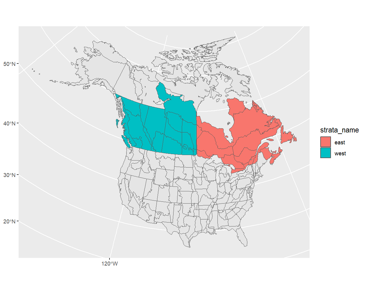
Stratify by custom stratification, using sf map object. For example, let’s look at an east/west divide of southern Canada with BBS CWS strata.
First we’ll start with the CWS BBS data
map <- load_map("bbs_cws")We’ll modify this by first looking only at provinces (omitting the northern territories), transforming to the GPS CRS (4326), and ensuring the resulting polygons are valid.
new_map <- map %>%
  filter(country_code == "CA", !prov_state %in% c("NT", "NU", "YT")) %>%
  st_transform(4326)%>%
  st_make_valid()
Now we can crop this map to make a western and an eastern portion, defined by longitude and latitude (which is why we first transformed to the GPS CRS).
west <- st_crop(new_map, xmin = -140, ymin = 42, xmax = -95, ymax = 68) %>%
  mutate(strata_name = "west")
#> Warning: attribute variables are assumed to be spatially constant throughout all geometries
east <- st_crop(new_map, xmin = -95, ymin = 42, xmax = -52, ymax = 68) %>%
  mutate(strata_name = "east")
#> Warning: attribute variables are assumed to be spatially constant throughout all geometries
Now we’ll bind these together and transform back to the original CRS
new_strata <- bind_rows(west, east) %>%
  st_transform(st_crs(map))

ggplot() +
  geom_sf(data = map) +
  geom_sf(data = new_strata, aes(fill = strata_name), alpha = 1)
Looks good! Let’s use it in our stratification and take a look at the points afterwards to ensure they’ve been categorized appropriately.
s <- stratify(by = "canada_ew", species = "Mallard",
              strata_custom = new_strata)
#> Using 'canada_ew' (custom) stratification
#> Loading BBS data...
#> Filtering to species Mallard (1320)
#> Stratifying data...
#> Preparing strata (ESRI:102008; North_America_Albers_Equal_Area_Conic)...
#>   Summarizing strata...
#>   Calculating area weights...
#>   Joining routes to spatial layer...
#>   Renaming routes...
#>   Omitting 110,107/127,482 surveys, on 3,812 unique routes that do not match a stratum.
#>     To see omitted routes use `return_omitted = TRUE` (see ?stratify)

s$meta_data
#> $stratify_by
#> [1] "canada_ew"
#>
#> $stratify_type
#> [1] "custom"
#>
#> $species
#> [1] "Mallard"
#>
#> $sp_aou
#> [1] 1320
routes <- s$routes_strata %>%
  st_as_sf(coords = c("longitude", "latitude"), crs = 4326)

ggplot() +
  geom_sf(data = new_strata, aes(fill = strata_name), alpha = 1) +
  geom_sf(data = routes, aes(shape = strata_name))